Head Motion Benchmark

Introduction

In this project, we used FiberFox to simulate entire dMRI series for ABCD, HCP, DSIQ5, and HASC55 data. Head motion was then introduced by applying rigid transforms to the streamline data (translations and rotations). Then, QSIPrep used both SHORELine and Eddy to estimate the introduced head motion — analysis of these results are evaluated in this notebook.

Libraries & Setup

The data are available on OSF at this link. This package internally downloads and cleans them for your convenience. They’re available preprocessed within the package:

# for viewing the preprocessed data
motion_df <- SHORELINEPaper::motion_df %>%
  as_tibble()
data("error_df_wsetting")
data("error_rmse_wsetting") # for analysis of estimated motion

Sample

The table below shows the number of b0’s for each scheme:

motion_df %>%
  filter(
    iternum == 1 &
      method == "SHORELine" &
      denoising == "none" &
      bval > 100 &
      setting == "Affine") %>%
  group_by(percent_motion, scheme) %>%
  summarise(max_b = max(bval),
            num_b = n()) %>%
  ungroup() %>%
  distinct(scheme, max_b, num_b) %>%
  t() %>%
  row_to_names(1) %>%
  data.frame() %>%
  add_row(ABCD = "Shelled", HCP = "Shelled", DSIQ5 = "Cartesian", HASC55 = "Random", .before = 1) -> tab1

## `summarise()` has grouped output by 'percent_motion'. You can override using
## the `.groups` argument.

rownames(tab1) <- c("Type", "Max. b", "Num. b > 0")

gt(tab1, rownames_to_stub = TRUE) %>%
  tab_header("Scheme properties and processing pipeline runs") %>%
  opt_table_font("Helvetica")

Scheme properties and processing pipeline runs
	ABCD	DSIQ5	HASC55	HCP
Type	Shelled	Cartesian	Random	Shelled
Max. b	3000	4985	5015	3010
Num. b > 0	96	257	55	270

Below is a breakdown of how the runs were accumulated:

motion_df %>%
  filter(volnum == 0) %>%
  select(Algorithm = method, Model = setting, Denoising = denoising, percent_motion, scheme) %>%
  group_by_all() %>%
  summarise(n = n()) %>%
  pivot_wider(names_from = scheme, values_from = n) %>%
  ungroup() %>%
  mutate(across(where(is.numeric), ~ ifelse(is.na(.), 0, .))) %>%
  mutate(Denoising = ifelse(Denoising == "none", "None", "MP-PCA")) %>%
  mutate(percent_motion = paste0(as.character(percent_motion), " %")) %>%
  # insert empty string for tidyness
  mutate(across(where(is.factor), as.character)) %>%
  group_by(Algorithm, Model, Denoising) %>%
  mutate_at(vars(Algorithm:Denoising), ~ replace(.x, duplicated(.x), "")) %>%
  ungroup() %>%
  select(-Algorithm) %>%
  gt() %>%
  tab_spanner("# Pipeline Runs", columns = ABCD:HASC55) %>%
  cols_align(align = "right", columns = percent_motion:HASC55) %>%
  tab_row_group(
    label = "Eddy",
    rows = 1:12
  ) %>%
  tab_row_group(
    label = "SHORELine",
    rows = 13:24
  ) %>%
  opt_table_font("Helvetica")

## `summarise()` has grouped output by 'Algorithm', 'Model', 'Denoising',
## 'percent_motion'. You can override using the `.groups` argument.

Model	Denoising	percent_motion	# Pipeline Runs
Model	Denoising	percent_motion	ABCD	HCP	DSIQ5	HASC55
SHORELine
Affine	MP-PCA	15 %	30	30	30	30
		30 %	30	30	30	30
		50 %	30	30	30	30
Affine	None	15 %	30	30	30	30
		30 %	30	30	30	30
		50 %	30	30	30	30
Rigid	MP-PCA	15 %	30	30	30	30
		30 %	30	30	30	30
		50 %	30	30	30	30
Rigid	None	15 %	30	30	30	30
		30 %	30	30	30	30
		50 %	30	30	30	30
Eddy
Linear	MP-PCA	15 %	30	30	0	0
		30 %	30	30	0	0
		50 %	30	30	0	0
Linear	None	15 %	30	30	0	0
		30 %	30	30	0	0
		50 %	30	30	0	0
Quadratic	MP-PCA	15 %	30	30	0	0
		30 %	30	30	0	0
		50 %	30	30	0	0
Quadratic	None	15 %	30	30	0	0
		30 %	30	30	0	0
		50 %	30	30	0	0

And finally the total scans and volumes:

motion_df %>%
  filter(volnum == 0) %>%
  select(Algorithm = method, Model = setting, Denoising = denoising, percent_motion, scheme) %>%
  group_by_all() %>%
  summarise(n = n()) %>%
  pivot_wider(names_from = scheme, values_from = n) %>%
  ungroup() %>%
  mutate(across(where(is.numeric), ~ ifelse(is.na(.), 0, .))) %>%
  mutate(Denoising = ifelse(Denoising == "none", "None", "MP-PCA")) %>%
  mutate(percent_motion = paste0(as.character(percent_motion), " %")) %>%
  group_by(Algorithm) %>%
  summarise(across(ABCD:HASC55,sum)) %>%
  gt() %>%
  tab_header("Total Scans") %>%
  opt_table_font("Helvetica")

## `summarise()` has grouped output by 'Algorithm', 'Model', 'Denoising',
## 'percent_motion'. You can override using the `.groups` argument.

Total Scans
Algorithm	ABCD	HCP	DSIQ5	HASC55
Eddy	360	360	0	0
SHORELine	360	360	360	360

motion_df %>%
  filter(bval > 0) %>%
  select(Algorithm = method, Model = setting, Denoising = denoising, percent_motion, scheme) %>%
  group_by(scheme) %>%
  summarise(`Total b > 0 Volumes` = n()) %>%
  t() %>%
  row_to_names(1) %>%
  data.frame() %>%
  gt(rownames_to_stub = TRUE) %>%
  opt_table_font("Helvetica")

	ABCD	DSIQ5	HASC55	HCP
Total b > 0 Volumes	69120	92520	19800	194400

Note that errors for rotation are converted from radians to degrees, and we also extract only the \(b > 0\) volumes. Both Eddy and SHORELine use different methods (non-GP and non-SHORE) for motion-correcting these images.

Motion Analysis

1. Is there an RMSE difference between the Rigid/Affine and Linear/Quadratic settings?

We tested Rigid and Affine transformation models for SHORELine and Linear and Quadratic models in Eddy. In Eddy, the models only affect Eddy current correction so we shouldn’t see a difference in head motion estimates. SHORELine may or may not benefit from having more degrees of freedom in the transformation model.

Here we test whether there are significant effects of transformation model. Under the hood R will pair the same scans and perform a paired t-test by subtracting alphabetically. For SHORELine this means Affine - Rigid and for Eddy it means Linear - Quadratic.

# TODO put these long functions into a function

# TODO Helvetica in the header and stub

setting_tests <- error_rmse_wsetting %>%
  rename(hmc_method=method) %>%
  group_by(denoising, scheme, motion.type, hmc_method, percent_motion) %>%
  do(test = tidy(t.test(rmse ~ setting, data=., paired=TRUE))) %>%
  unnest(test)

# Adjust the p-values and order them by the largest absolute effects
setting_tests_adj <- setting_tests %>% 
  select(!c(parameter, method, alternative)) %>%
  
  pivot_wider(
    names_from = motion.type, 
    values_from = c(estimate:conf.high)
    ) %>%
  
  # p adjust any pvalues
  mutate(
    across(
      contains("p.value"),
       ~p.adjust(.x),
      .names = "Adjusted_{.col}"
      )
    ) %>%

  # filter sig pvals
  # no eddy rows should get through this filter
  filter(if_any(contains("Adjusted"), ~.x < 0.01))

setting_tests_adj %>%
  select(Method = hmc_method, Scheme = scheme, Denoising = denoising, percent_motion, everything()) %>%      
  # reorder columns
  arrange(Method, Scheme, Denoising) %>%
  
  # convert to char for empty strings &
  # insert empty strings for every group where the values are duplicated
  # for clarity
  
  mutate(across(where(is.factor), as.character)) %>%
  mutate(percent_motion=paste0(percent_motion,"%")) %>%
  group_by(Method, Scheme, Denoising) %>%
  mutate_at(vars(Method:Denoising), ~ replace(.x, duplicated(.x), "")) %>%
  ungroup() %>%
  
  # precision for the confidence intervals that get merged
  mutate(across(contains("conf"), ~ round(.x, 2))) %>%
  select(!matches("^p.value")) %>%
  
  # last details
  mutate(Denoising = ifelse(Denoising == "none", "None", "DWIDenoise")) %>%
  
  
  gt(rowname_col = "Scheme") -> setting_tests_gt
  
setting_tests_gt %>%
  tab_spanner(label = md("*Rotation*"), columns = matches("Rotation")) %>%
  tab_spanner(label = md("*Translation*"), columns = matches("Translation")) %>%
  
  # string format confidence intervals
  cols_merge(columns = c(conf.low_Translation, conf.high_Translation), pattern = "[{1}, {2}]") %>%
  cols_label(
    conf.low_Translation = "95% CI"
  ) %>%
  cols_merge(columns = c(conf.low_Rotation, conf.high_Rotation), pattern = "[{1}, {2}]") %>%
  cols_label(
    conf.low_Rotation = "95% CI"
  ) %>%
  fmt(
    columns = matches("p.value"),
    fns = function(x){
      format.pval(x, eps=0.0001, digits = 3)
    }
  ) %>%
  fmt_number(
    columns = matches("statistic|estimate"),
    decimals = 3
  ) %>%
  cols_label(
    Adjusted_p.value_Rotation = md("Adj. *p*-value"),
    Adjusted_p.value_Translation = md("Adj. *p*-value"),
    estimate_Rotation = md("Estimate"),
    estimate_Translation = md("Estimate"),
    statistic_Rotation = md("Statistic"),
    statistic_Translation = md("Statistic"),
    percent_motion = md("Motion Prevalence")
  ) %>%
  
  data_color(
    columns = c(estimate_Translation, estimate_Rotation),
    colors = scales::col_numeric(
      palette = rocket(10),
      domain = c(-0.1, 0.5)
    )
  ) %>%
  tab_style(
    style = list(
      cell_text(font = "Helvetica")
      ),
    locations = cells_body(
      columns = everything(),
      rows = everything()
    )
  ) %>%
  tab_style(
    style = list(
      cell_text(weight = "bold")
      ),
    locations = cells_column_labels(columns = everything())
  ) %>%
  tab_style(
    style = list(
      cell_text(weight = "bold")
      ),
    locations = cells_column_spanners(spanners = everything())
  ) %>%
  tab_header(md("**Predicting RMSE of Motion Estimates**"),
             subtitle = "Evaluation of Effects on Transformation") %>%
  opt_table_font("Helvetica")

Predicting RMSE of Motion Estimates
Evaluation of Effects on Transformation
	Method	Denoising	Motion Prevalence	Rotation				Translation
	Method	Denoising	Motion Prevalence	Estimate	Statistic	95% CI	Adj. p-value	Estimate	Statistic	95% CI	Adj. p-value
ABCD	SHORELine	DWIDenoise	15%	0.247	13.695	[0.21, 0.28]	<1e-04	−0.032	−9.312	[-0.04, -0.03]	<1e-04
		DWIDenoise	30%	0.135	10.929	[0.11, 0.16]	<1e-04	−0.044	−11.353	[-0.05, -0.04]	<1e-04
		DWIDenoise	50%	0.095	11.360	[0.08, 0.11]	<1e-04	0.054	0.479	[-0.18, 0.29]	1.0000
ABCD	SHORELine	None	15%	0.252	13.859	[0.21, 0.29]	<1e-04	−0.036	−11.397	[-0.04, -0.03]	<1e-04
		DWIDenoise	30%	0.144	11.774	[0.12, 0.17]	<1e-04	−0.047	−11.954	[-0.05, -0.04]	<1e-04
		DWIDenoise	50%	0.088	10.640	[0.07, 0.11]	<1e-04	−0.060	−13.451	[-0.07, -0.05]	<1e-04
HCP	SHORELine	DWIDenoise	15%	0.417	40.240	[0.40, 0.44]	<1e-04	−0.038	−18.948	[-0.04, -0.03]	<1e-04
		DWIDenoise	30%	0.259	19.352	[0.23, 0.29]	<1e-04	−0.033	−13.796	[-0.04, -0.03]	<1e-04
		DWIDenoise	50%	0.124	9.790	[0.10, 0.15]	<1e-04	−0.026	−12.963	[-0.03, -0.02]	<1e-04
HCP	SHORELine	None	15%	0.425	39.922	[0.40, 0.45]	<1e-04	−0.040	−19.837	[-0.04, -0.04]	<1e-04
		DWIDenoise	30%	0.265	18.940	[0.24, 0.29]	<1e-04	−0.033	−14.515	[-0.04, -0.03]	<1e-04
		DWIDenoise	50%	0.125	9.735	[0.10, 0.15]	<1e-04	−0.026	−13.125	[-0.03, -0.02]	<1e-04
DSIQ5	SHORELine	DWIDenoise	15%	0.086	11.138	[0.07, 0.10]	<1e-04	−0.003	−1.445	[-0.01, 0.00]	1.0000
		DWIDenoise	30%	0.055	8.305	[0.04, 0.07]	<1e-04	0.071	0.931	[-0.09, 0.23]	1.0000
		DWIDenoise	50%	0.042	6.898	[0.03, 0.05]	<1e-04	−0.001	−0.361	[-0.01, 0.01]	1.0000
DSIQ5	SHORELine	None	15%	0.092	11.753	[0.08, 0.11]	<1e-04	−0.003	−1.786	[-0.01, 0.00]	1.0000
		DWIDenoise	30%	0.056	8.261	[0.04, 0.07]	<1e-04	−0.005	−1.692	[-0.01, 0.00]	1.0000
		DWIDenoise	50%	0.043	6.183	[0.03, 0.06]	<1e-04	0.001	0.253	[-0.01, 0.01]	1.0000
HASC55	SHORELine	DWIDenoise	15%	0.153	11.189	[0.12, 0.18]	<1e-04	−0.004	−1.028	[-0.01, 0.00]	1.0000
		DWIDenoise	30%	0.115	7.723	[0.08, 0.15]	<1e-04	−0.010	−3.373	[-0.02, 0.00]	0.0489
		DWIDenoise	50%	0.087	6.415	[0.06, 0.11]	<1e-04	−0.022	−3.811	[-0.03, -0.01]	0.0167
HASC55	SHORELine	None	15%	0.214	10.330	[0.17, 0.26]	<1e-04	0.008	1.183	[-0.01, 0.02]	1.0000
		DWIDenoise	30%	0.123	7.457	[0.09, 0.16]	<1e-04	−0.004	−0.907	[-0.01, 0.00]	1.0000
		DWIDenoise	50%	0.086	6.134	[0.06, 0.12]	<1e-04	−0.017	−3.517	[-0.03, -0.01]	0.0350

We can see that all the effects that survive a filter for \(\text{Adjusted-}p < 0.01\) are for SHORELine and the estimates are positive. This means that Affine RMSE is greater than Rigid RMSE. Although these estimates are all tiny, we will simplify subsequent comparisons by only choosing rigid. Rigid also has the benefit of much shorter run times than Affine. As expected, there are no differences for Eddy.

We’ll subset the RMSE values to just those we’re using for the rest of the comparisons:

# Only look at one setting per method
error_rmse <- error_rmse_wsetting %>% 
  filter(setting %in% c("Rigid", "Quadratic")) %>%
  select(-setting)

2. Summarization of Motion Detection Errors

Here we summarize how big errors were in estimating head motion. We first look at the distribution of errors to check that it’s centered around zero, and that this is the case for both eddy and shoreline.

# TODO generally improve this plot

error_df_wsetting %>%
  select(method, scheme, denoising, percent_motion, motion.type, Error = value) %>%
  filter(Error < 20 & Error > -20) %>% # very egregious errors
  mutate(percent_motion = ordered(percent_motion, levels=c(50, 30, 15))) %>%
  ggplot(aes(x=Error, y=percent_motion, fill=scheme)) +
  stat_slab(alpha = 0.5, width = 0, .width = 0, point_colour = NA, expand=TRUE, color = "black") +
  facet_grid(method ~ motion.type, scales = "free") +
  ggtitle("Distribution of Motion Estimate Errors")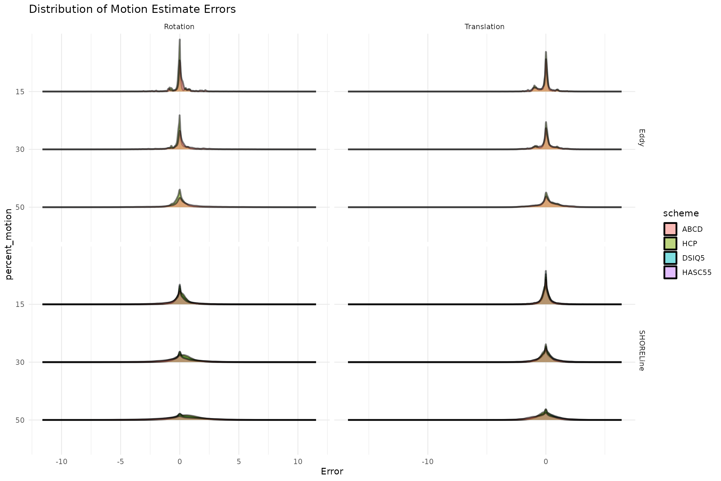

Next we see what the standard deviation of the error is. This tells us, on average, the amount of degrees or mm we can expect an error to be for each method.

# TODO put formatting into a function

rmse_summaries <- error_rmse %>%
  group_by(denoising, scheme, motion.type, method, percent_motion) %>%
  summarise(mean_rmse=mean(rmse), 
            sd_rmse=sd(rmse), 
            se_rmse=sd_rmse/sqrt(length(rmse)),
            group_mean_error=mean(mean_error),
            sd_mean_error=sd(mean_error))

## `summarise()` has grouped output by 'denoising', 'scheme', 'motion.type',
## 'method'. You can override using the `.groups` argument.

rmse_summaries <- rmse_summaries %>%
  mutate(
    motion.type = case_when(
      str_detect(motion.type, "Rotation")  ~ "Rotation (degrees)",
      str_detect(motion.type, "Translation")  ~ "Translation (mm)"
      ),
    Denoising=case_when(denoising == "none"  ~ "None", TRUE ~ "MP-PCA") %>% factor()
    
  )

pd=position_dodge2(width=0.7, preserve="single")
linetypes = c("None" = 1, "MP-PCA" = 2)

error_mean_plt <-  ggplot(
    rmse_summaries %>% mutate(percent_motion=paste0(percent_motion, "%")),
    aes(
      y=group_mean_error, x=percent_motion, 
      fill=method, group=Denoising)
    ) +
  geom_bar(aes(alpha=Denoising), stat="identity", position=pd, width = 0.6) +
  geom_errorbar(
    aes(ymax=group_mean_error+mean_rmse,
        ymin=group_mean_error-mean_rmse,
        width=0.7),
    color = "black", position=pd
    ) +
  facet_grid(motion.type~scheme, scales="free") + 
  scale_color_manual(
    values=c("SHORELine"="#d95f02", "Eddy"="#1b9e77"), guide="none"
    ) +
  scale_fill_manual(
    values=c("SHORELine"="#d95f02", "Eddy"="#1b9e77")
    ) +
  scale_alpha_manual(
    name="Denoising Strategy",
    values=c(1.0, 0.5)
    ) +
  theme_bw(
    base_family="Helvetica",
    base_size=12
  ) +
  labs(title = "Head Motion Estimate Error", 
       y = "Mean Error (±Mean RMSE)", 
       x = "Motion Prevalence", 
       fill = "Method"
       ) +
  guides(linetype=guide_legend(override.aes=list(fill=NA)))

# TODO reduce plot size, increase font size
error_mean_plt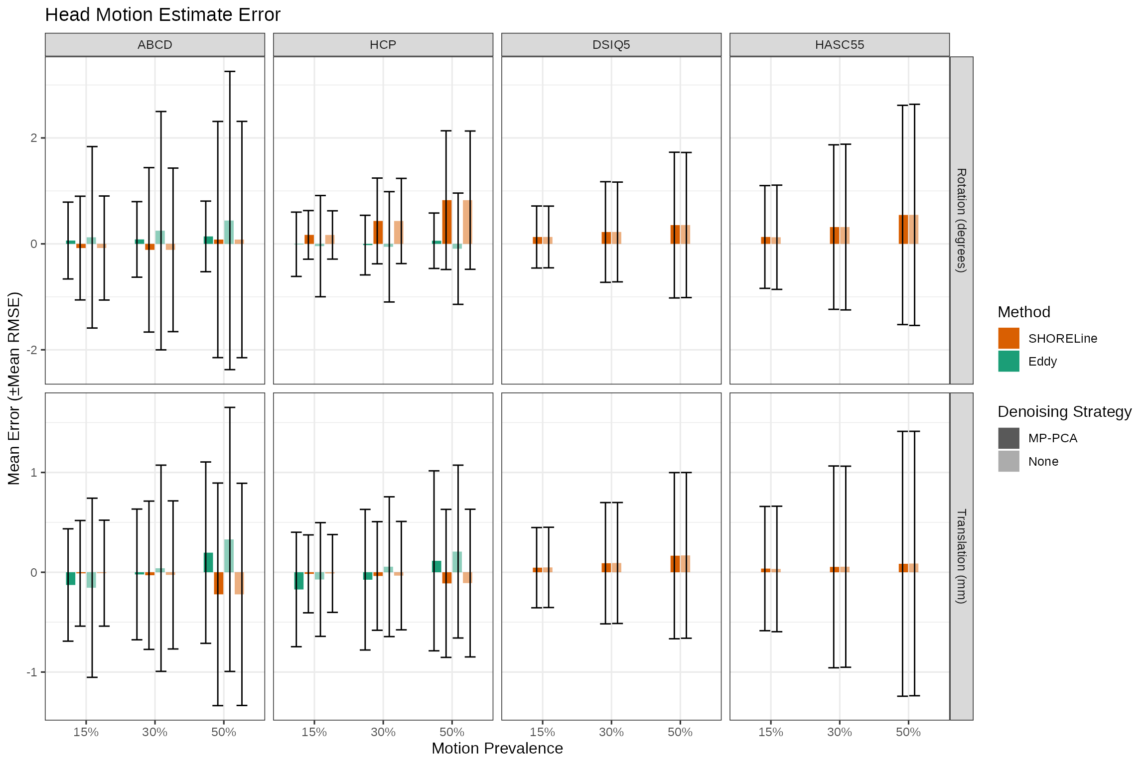

# Summarize the motion rmse in the different cells
# rmse_plt <-  ggplot(
#     rmse_summaries,
#     aes(
#       y=mean_rmse, x=percent_motion, 
#       color=method, fill=method)
#     ) +
#   geom_bar(aes(alpha=Denoising), stat="identity", position=pd, width = 0.6) +
#   geom_errorbar(
#     aes(ymax=mean_rmse+sd_rmse, ymin=mean_rmse-sd_rmse,
#         width=0.6),
#     color = "black", position=pd
#     ) +
#   facet_grid(motion.type~scheme, scales="free") + 
#   scale_color_manual(
#     values=c("SHORELine"="#d95f02", "Eddy"="#1b9e77"), guide="none"
#     ) +
#   scale_fill_manual(
#     values=c("SHORELine"="#d95f02", "Eddy"="#1b9e77")
#     ) +
#   scale_alpha_manual(
#     name="Denoising Strategy",
#     values=c(1.0, 0.5)
#     ) +
#   theme_bw(
#     base_family="Helvetica",
#     base_size=12
#   ) +
#   labs(title = "Motion Estimate RMSE",
#        y = "Mean RMSE (±SD)", 
#        x = "Percent Motion Volumes", 
#        fill = "Method",
#        ) +
#   guides(linetype=guide_legend(override.aes=list(fill=NA)))


rmse_plt <-  ggplot(
    rmse_summaries %>% mutate(percent_motion=paste0(percent_motion, "%")),
    aes(
      y=mean_rmse, x=percent_motion, 
      fill=method, group=Denoising)
    ) +
  geom_bar(aes(alpha=Denoising), stat="identity", position=pd, width = 0.6) +
  geom_errorbar(
    aes(ymax=mean_rmse+sd_rmse, ymin=mean_rmse-sd_rmse,
        width=0.6),
    color = "black", position=pd
    ) +
  facet_grid(motion.type~scheme, scales="free") + 
  scale_fill_manual(
    values=c("SHORELine"="#d95f02", "Eddy"="#1b9e77")
    ) +
  scale_alpha_manual(
    name="Denoising Strategy",
    values=c(1.0, 0.5)
    ) +
  theme_bw(
    base_family="Helvetica",
    base_size=12
  ) +
  labs(title = "Motion Estimate RMSE",
       y = "Mean RMSE (±SD)", 
       x = "Motion Prevalence", 
       fill = "Method",
       ) +
  guides(linetype=guide_legend(override.aes=list(fill=NA)))

rmse_plt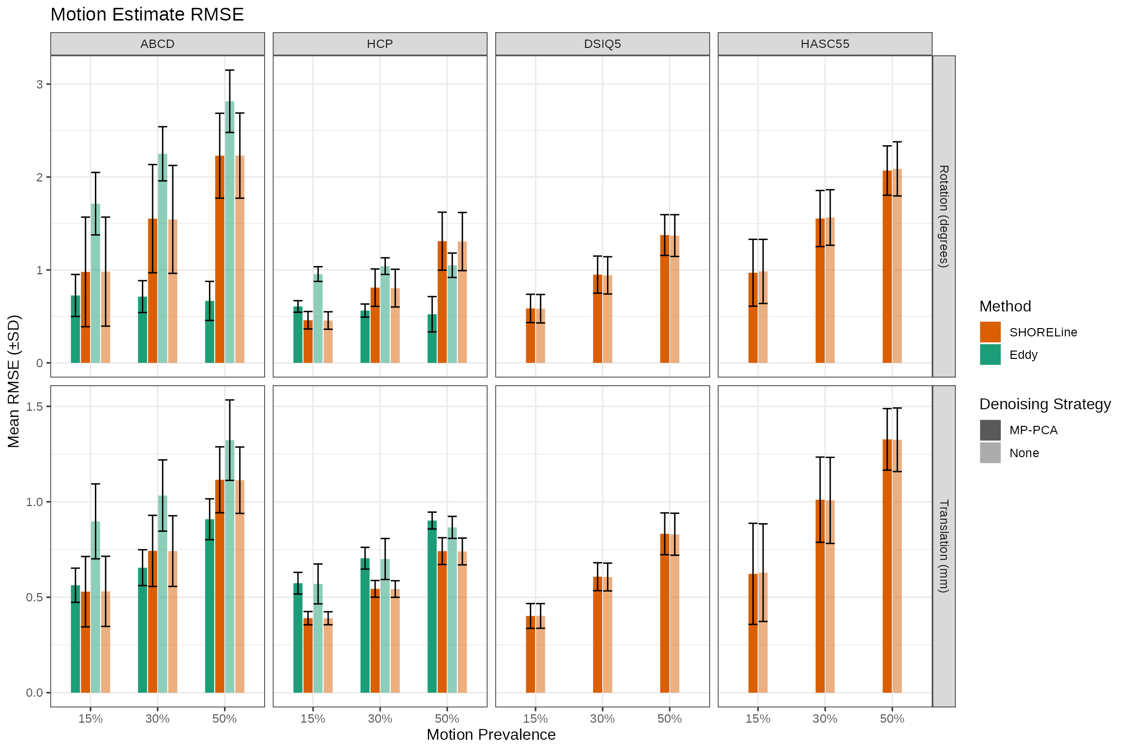

Here is how means were reported in the paper, and also how they were calculated for the OHBM poster.

# TODO formatting
errs <- error_rmse %>% group_by(motion.type) %>% 
  summarise(mean_mean_error=mean(mean_error),
            sd_mean_error=sd(mean_error))

errs %>%
  gt() %>%
  tab_header("Mean RMSE by Motion Type") %>%
  opt_table_font("Helvetica")

Mean RMSE by Motion Type
motion.type	mean_mean_error	sd_mean_error
Rotation	0.19375489	0.3876132
Translation	0.01237718	0.1987452

3. Compare Performance on Sampling Schemes

There are 4 sampling schemes compared here. How well do the motion correction methods work on each?

rmse_summaries_collapsed <- error_rmse %>%
  group_by(scheme, motion.type, method, denoising) %>%
  summarise(mean_rmse=mean(rmse), 
            sd_rmse=sd(rmse), 
            se_rmse=sd_rmse/sqrt(length(rmse)),
            group_mean_error=mean(mean_error),
            sd_mean_error=sd(mean_error)) %>%
  mutate(denoised = recode(denoising, none="", dwidenoise="+ MP-PCA"),
         method_name = paste(method, denoised)) %>%
  select(-denoised) %>%
  filter(method_name != "SHORELine + MP-PCA") # no difference, so skip it

## `summarise()` has grouped output by 'scheme', 'motion.type', 'method'. You can
## override using the `.groups` argument.

rmse_summaries_collapsed %>%
  ungroup() %>%
  mutate(
    num_directions = case_when(
      scheme == "ABCD"    ~ 103,
      scheme == "HCP"     ~ 270,
      scheme == "DSIQ5"   ~ 257,
      scheme == "HASC55"  ~ 55
    )
  ) %>%
# rmse_summaries_collapsed$num_directions <- recode(
#   rmse_summaries_collapsed$scheme,
#   ABCD=103,
#   HCP=270,
#   DSIQ5=257,
#   HASC55=55)

  mutate(
    denoiser = case_when(
      denoising == "none" ~ "None",
      TRUE                ~ "MP-PCA"
    )
  ) %>%
# rmse_summaries_collapsed$denoiser <- recode(
#   rmse_summaries_collapsed$denoising,
#   none="None",
#   dwidenoise="MP-PCA"
# )

  mutate(
    scheme_type = case_when(
      str_detect(scheme, "ABCD|HCP")  ~ "Shelled",
      TRUE                            ~ "Non-Shelled"
    )
  ) %>%
  
# rmse_summaries_collapsed$scheme_type = recode(
#   rmse_summaries_collapsed$scheme,
#   ABCD="Shelled",
#   HCP="Shelled",
#   DSIQ5="Non-Shelled",
#   HASC55="Non-Shelled")

  mutate(
    motion.type = case_when(
      str_detect(motion.type, "Rotation")     ~ "Rotation (degrees)",
      str_detect(motion.type, "Translation")  ~ "Translation (mm)",
    )
  ) -> rmse_summaries_collapsed
# rmse_summaries_collapsed$motion.type <- recode(
#   rmse_summaries_collapsed$motion.type,
#   Rotation="Rotation (degrees)",
#   Translation="Translation (mm)"
#   )

# Summarize the motion rmse in the different cells
pd2 = position_dodge(8)
directions_plt <-  ggplot(
    rmse_summaries_collapsed,
    aes(x=num_directions, y=mean_rmse,
        color=method,
        shape=scheme_type,
        linetype=denoiser,
        group=method_name)) +
  geom_errorbar(
    aes(ymax=mean_rmse+sd_rmse, ymin=mean_rmse-sd_rmse), 
    position=pd2) +
  geom_point(size=2, position=pd2) +
  geom_line() +
  facet_grid(motion.type~.) +
  theme_bw(
    base_family="Helvetica",
    base_size=12
  ) +
  scale_color_manual(
    labels=c("SHORELine", "Eddy"),
    values=c("SHORELine"="#d95f02", "Eddy"="#1b9e77")) +
  scale_linetype_manual(values=c("None"=1,"MP-PCA" = 2)) +
  labs(title = "RMSE by Scheme Type", 
       y = "Mean RMSE (±SD)", 
       x = "Number of Directions", 
       color = "Method",
       linetype= "Denoising\nMethod",
       shape="Scheme\nType")

directions_plt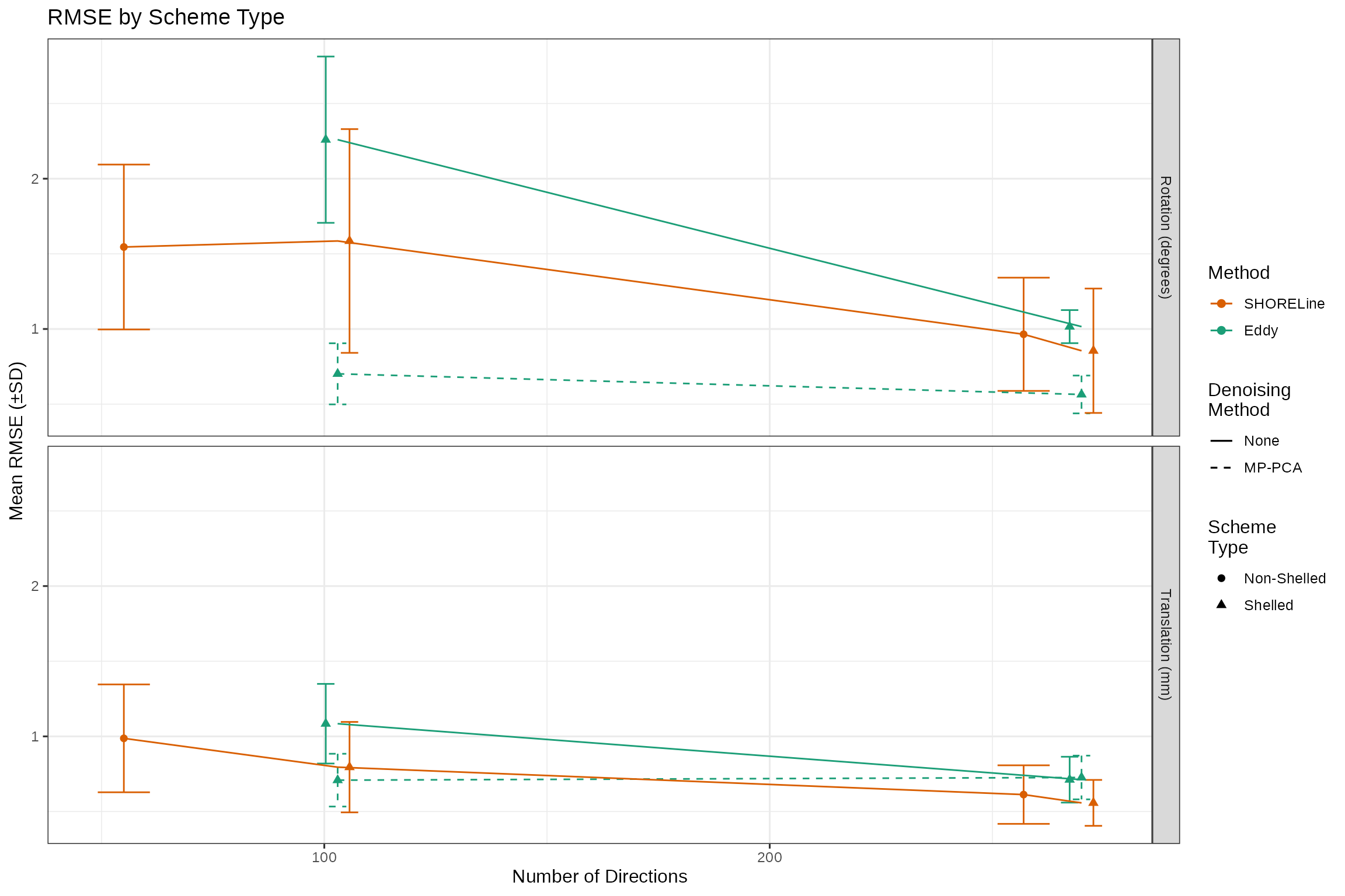

This is just another view of the previous plot, but interesting in that it clearly shows that SHORELine’s performance on the 55-direction CS-DSI scan is in the range of the performance on the ABCD multi shell scheme, which has almost twice as many directions. We can statistically test this, to be sure:

error_rmse_dirs <- error_rmse

error_rmse_dirs$num_directions <- recode(
  error_rmse_dirs$scheme,
  ABCD=103,
  HCP=270,
  DSIQ5=257,
  HASC55=55)

error_rmse_dirs$scheme_type = recode(
  error_rmse_dirs$scheme,
  ABCD="Shelled",
  HCP="Shelled",
  DSIQ5="Non-Shelled",
  HASC55="Non-Shelled")

# Convert to percentage values
error_rmse_dirs$percent_motion <- with(
  error_rmse_dirs,
  as.numeric(levels(percent_motion))[percent_motion])

error_rmse_dirs <- error_rmse_dirs %>%
  # make it presentable for the table
  mutate(
    Denoising = case_when(
      denoising == "dwidenoise"  ~ "MP-PCA",
      TRUE                       ~ "None"
    ),
    `Scheme Type` = scheme_type,
    `Motion Prevalence` = percent_motion,
    RMSE = rmse,
    `N. Directions` = num_directions,
    Method = method
  )

# run lm
# rotation_shell_model <- lm(
#   RMSE ~ Method + `Scheme Type` * `N. Directions` + Denoising + `Motion Prevalence`,
#   data=subset(error_rmse_dirs, motion.type=="Rotation"))
# 
# translation_shell_model <- lm(
#   RMSE ~ Method + `Scheme Type` * `N. Directions`+ Denoising + `Motion Prevalence`,
#   data=subset(error_rmse_dirs, motion.type=="Translation"))

rotation_shell_model <- lm(
  RMSE ~ `Scheme Type` * `N. Directions` + Denoising + `Motion Prevalence`,
  data=subset(error_rmse_dirs, motion.type=="Rotation"))

translation_shell_model <- lm(
  RMSE ~ `Scheme Type` * `N. Directions`+ Denoising + `Motion Prevalence`,
  data=subset(error_rmse_dirs, motion.type=="Translation"))

# create gt tables
translation_rmse_tab <- tbl_regression(
  translation_shell_model, 
  intercept=TRUE,
  estimate_fun = ~style_number(.x, digits=3)
  ) %>%
  bold_p() %>%
  bold_labels() %>% 
  italicize_levels()

rotation_rmse_tab <- tbl_regression(
  rotation_shell_model, 
  intercept=TRUE,
  estimate_fun = ~style_number(.x, digits=3)
  ) %>%
  bold_p() %>%
  bold_labels() %>% 
  italicize_levels()

capt <- "**Supplementary Listing 1: _Factors Impacting RMSE Following Head Motion Correction_**. Error following motion correction is largely due to uncontrolled factors (presupposed head motion), preprocessing choices (use of denoising), and experimental design (sampling scheme)."

# merge and display

rmse_model_table <- tbl_merge(list(translation_rmse_tab, rotation_rmse_tab), tab_spanner = c("Translation", "Rotation")) %>%
  as_gt() %>%
  fmt_number(n_sigfig = 2, matches("Beta"), force_sign = TRUE) %>%
  tab_header(title = "Predicting RMSE of Estimated Motion",
             #subtitle = "Main Effects of Denoising, Number of Directions, and Percent Motion, including interactions with Shell Scheme Type"
             ) %>%
  # tab_source_note(md(capt)) %>%
  # tab_style(
  #   style = cell_text(
  #     size = "large"
  #   ),
  #   locations = cells_source_notes()
  # ) %>%
  opt_table_font("Helvetica")
  
  

rmse_model_table

Predicting RMSE of Estimated Motion
Characteristic	Translation			Rotation
Characteristic	Beta	95% CI¹	p-value	Beta	95% CI¹	p-value
(Intercept)	0.528	0.487, 0.569	<0.001	1.125	1.019, 1.231	<0.001
Scheme Type
Shelled	—	—		—	—
Non-Shelled	0.115	0.068, 0.161	<0.001	-0.278	-0.398, -0.157	<0.001
N. Directions	-0.001	-0.001, -0.001	<0.001	-0.004	-0.005, -0.004	<0.001
Denoising
MP-PCA	—	—		—	—
None	0.060	0.039, 0.081	<0.001	0.335	0.280, 0.391	<0.001
Motion Prevalence	0.013	0.012, 0.014	<0.001	0.021	0.019, 0.023	<0.001
Scheme Type * N. Directions
Non-Shelled * N. Directions	-0.001	-0.001, 0.000	<0.001	0.001	0.001, 0.002	<0.001
¹ CI = Confidence Interval

# save
rmse_model_table %>% gtsave(here("figures", "rmse_model_nomethod.pdf"), zoom=1)

A couple interesting results come out here along with some obvious ones. First, there is a main effect of the number of directions. The more directions, the smaller the RMSE.

4 Head to head comparison of SHORELine vs Eddy

The ABCD and HCP sequences are the only two schemes we tested that can be processed by both Eddy and SHORELine.

# Match the Eddy and SHORELine errors 
paired_error <- error_rmse %>%
  select(-mean_error, -sd_error) %>%
  filter(scheme %in% c("ABCD", "HCP")) %>%
  spread(method, rmse, sep="_") %>% 
  group_by(scheme, motion.type) %>% 
  mutate(shore_difference=method_Eddy - method_SHORELine) %>%
  
  # make it presentable for the table
  mutate(
    Denoising = case_when(
      denoising == "dwidenoise"  ~ "MP-PCA",
      TRUE                       ~ "None"
    ),
    Scheme = scheme,
    `Motion Type` = motion.type,
    `Motion Prevalence` = as.numeric(levels(percent_motion))[percent_motion]
  )

rotation_rmse_model_paired <- lm(
  shore_difference ~ Scheme * Denoising * `Motion Prevalence`,
  data=subset(paired_error, `Motion Type`=="Rotation"))

translation_rmse_model_paired <- lm(
  shore_difference ~ Scheme * Denoising * `Motion Prevalence`,
  data=subset(paired_error, `Motion Type`=="Translation"))

translation_rmse_paired_tab <- tbl_regression(
  translation_rmse_model_paired, 
  intercept=TRUE,
  estimate_fun = ~style_number(.x, digits=3)
  ) %>%
  bold_p() %>%
  bold_labels() %>% 
  italicize_levels()

rotation_rmse_paired_tab <- tbl_regression(
  rotation_rmse_model_paired, 
  intercept=TRUE,
  estimate_fun = ~style_number(.x, digits=3)
  ) %>%
  bold_p() %>%
  bold_labels() %>% 
  italicize_levels()

capt <- "**Supplementary Listing 2: _Comparing Eddy & SHORELine RMSE_**. The SHORELine RMSE value was subtracted from the Eddy RMSE from each simulated scan, and this difference was the outcome variable of the model. Positive Beta estimates suggest better performance by SHORELine. SHORELine shows less error than Eddy for all scenarios without denoising, but Eddy showed slightly superior performence when data was first denoised with MP-PCA."

tbl_merge(list(translation_rmse_paired_tab, rotation_rmse_paired_tab), tab_spanner = c("Translation", "Rotation")) %>%
  as_gt() %>%
  fmt_number(n_sigfig = 2, matches("Beta"), force_sign = TRUE) %>%
  tab_header(title = "Predicting RMSE Difference (Eddy — SHORELine) in ABCD & HCP Schemes",
             #subtitle = "Main Effects of Denoising & Percent Motion, and interactions with Shell Scheme"
             ) %>%
  # tab_source_note(md(capt)) %>%
  # tab_style(
  #   style = cell_text(
  #     size = "large"
  #   ),
  #   locations = cells_source_notes()
  # ) %>% 
  opt_table_font("Helvetica") -> rmse_difference_table

rmse_difference_table

Predicting RMSE Difference (Eddy — SHORELine) in ABCD & HCP Schemes
Characteristic	Translation			Rotation
Characteristic	Beta	95% CI¹	p-value	Beta	95% CI¹	p-value
(Intercept)	0.129	0.042, 0.216	0.004	0.297	0.056, 0.538	0.016
Scheme
ABCD	—	—		—	—
HCP	0.059	-0.065, 0.182	0.3	0.254	-0.087, 0.595	0.14
Denoising
MP-PCA	—	—		—	—
None	0.302	0.178, 0.425	<0.001	0.512	0.171, 0.853	0.003
Motion Prevalence	-0.007	-0.009, -0.004	<0.001	-0.037	-0.044, -0.030	<0.001
Scheme * Denoising
HCP * None	-0.286	-0.460, -0.112	0.001	-0.215	-0.697, 0.267	0.4
Scheme * Motion Prevalence
HCP * Motion Prevalence	0.006	0.003, 0.010	<0.001	0.011	0.001, 0.020	0.034
Denoising * Motion Prevalence
None * Motion Prevalence	0.002	-0.001, 0.006	0.2	0.033	0.023, 0.043	<0.001
Scheme * Denoising * Motion Prevalence
HCP * None * Motion Prevalence	-0.003	-0.008, 0.002	0.2	-0.028	-0.042, -0.014	<0.001
¹ CI = Confidence Interval

rmse_difference_table %>% gtsave(here("figures", "rmse_diff_model.pdf"), zoom=1)

We plot the RMSE differences:

ggplot(paired_error, 
       aes(x=paste0(percent_motion,"%"), 
           y=shore_difference,
           fill=denoising)) +
  stat_halfeye(
    justification = -.2,
    alpha = 0.8,
    .width = 0, 
    point_colour = NA) +
  geom_boxplot(
    width = .12, 
    outlier.shape = NA ## `outlier.shape = NA` works as well
  ) +
  # geom_point(
  #   ## draw horizontal lines instead of points
  #   shape = 95,
  #   size = 10,
  #   alpha = 0.2,
  # ) +
  coord_cartesian(xlim = c(1.2, NA)) +
  facet_grid(motion.type~scheme, scales="free") +
  scale_fill_manual(
    labels=c("MP-PCA", "None"),
    values=c("dwidenoise"="#FFC20A", "none"="#0C7BDC")) +
  theme_bw(
    base_family="Helvetica",
    base_size=12) +
  labs(
    title = "Differences in Estimate Error (Eddy - SHORELine)",
    y = "Estimation Error Difference",
    x = "Motion Prevalence",
    fill="Denoising\nMethod")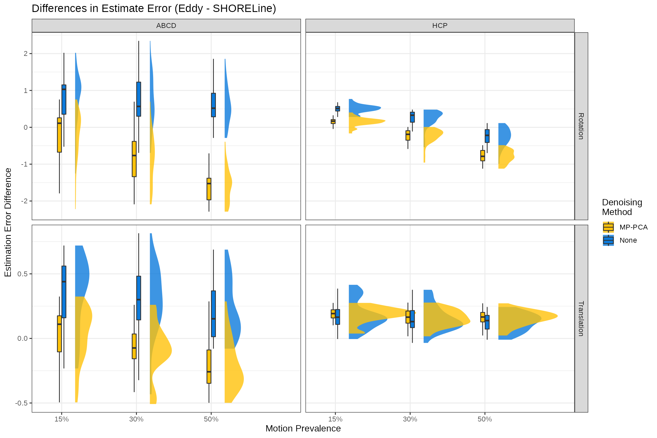

QC metric comparisons between SHORELine and Eddy

While accurately estimating head motion parameters is important, head motion is not the only artifact present in the simulated data. Other factors like eddy current distortion can impact the final quality of the results.

We therefore calculated and compared the Neighboring DWI Correlation (NDC) and FWHM of the final outputs between the two methods. The NDC and FWHM of the results are related, so we used the same method as in Cieslak et al. 2021 where FWHM is partialled out from the NDC measurements.

1. Test the Settings

data("qc_df")

Above we tested the settings to see if Linear/Quadratic or Rigid/Affine made a difference on motion estimation accuracy. Linear/Quadratic showed no difference, but Rigid performed better than Affine.

setting_tests <- qc_df %>%
  rename(hmc_method=method) %>%
  group_by(denoising, scheme, hmc_method, percent_motion) %>%
  do(test = tidy(t.test(ndc.corrected ~ setting, data=., paired=TRUE))) %>%
  unnest(test)

# Adjust the p-values and order them by the largest absolute effects
setting_tests <- setting_tests %>%
  mutate(p.value.adj = p.adjust(p.value))
# 
# significant.effects <- subset(setting_tests, (p.value.adj < 0.01))
# significant.effects[order(-abs(significant.effects$estimate)),]

setting_tests_gt <- setting_tests %>% 
  select(!c(parameter, method, alternative)) %>%
  select(Method = hmc_method, Scheme = scheme, Denoising = denoising, percent_motion, everything()) %>%
  arrange(Method, Scheme, Denoising) %>%
  
  # convert to char for empty strings &
  # insert empty strings for every group where the values are duplicated
  # for clarity
  
  mutate(across(where(is.factor), as.character)) %>%  
  group_by(Method, Scheme, Denoising) %>%
  mutate_at(vars(Method:Denoising), ~ replace(.x, duplicated(.x), "")) %>%
  ungroup() %>%
  
  # precision for the confidence intervals that get merged
  mutate(across(contains("conf"), ~ round(.x, 2))) %>%
  
  # last details
  mutate(Denoising = ifelse(Denoising == "none", "None", "DWIDenoise")) %>%
  select(-p.value) %>%
  mutate(pval_marker = p.value.adj) %>%
  mutate(percent_motion = paste0(as.character(percent_motion), " %")) %>%
  
  gt(rowname_col = "Scheme")

setting_tests_gt %>%
  cols_merge(columns = c(conf.low, conf.high), pattern = "[{1}, {2}]") %>%
  cols_label(
    conf.low = "95% CI"
  ) %>%
  fmt(
    columns = matches("p.value.adj"),
    fns = function(x){
      format.pval(x, eps=0.0001, digits = 3)
    }
  ) %>%
  tab_style(
    style = list(
      cell_text(weight = "bold")
      ),
    locations = cells_body(columns = p.value.adj, rows = pval_marker < 0.01)
  ) %>%
  fmt_number(
    columns = matches("statistic|estimate"),
    decimals = 3
  ) %>%
  cols_label(
    p.value.adj = md("Adj. *p*-value"),
    estimate = md("Estimate"),
    statistic = md("Statistic"),
    percent_motion = md("% Motion")
  ) %>%
  tab_style(
    style = list(
      cell_text(weight = "bold")
      ),
    locations = cells_column_labels(columns = everything())
  ) %>%
  opt_table_font("Helvetica")

	Method	Denoising	% Motion	Estimate	Statistic	95% CI	Adj. p-value	pval_marker
ABCD	SHORELine	DWIDenoise	15 %	0.014	11.039	[0.01, 0.02]	<1e-04	2.139571e-10
		DWIDenoise	30 %	0.014	8.523	[0.01, 0.02]	<1e-04	6.077568e-08
		DWIDenoise	50 %	0.015	6.856	[0.01, 0.02]	<1e-04	4.233490e-06
ABCD	SHORELine	DWIDenoise	15 %	0.015	8.628	[0.01, 0.02]	<1e-04	4.985773e-08
		DWIDenoise	30 %	0.015	10.274	[0.01, 0.02]	<1e-04	1.103746e-09
		DWIDenoise	50 %	0.015	5.777	[0.01, 0.02]	<1e-04	7.644406e-05
HCP	SHORELine	DWIDenoise	15 %	0.017	30.747	[0.02, 0.02]	<1e-04	3.959222e-22
		DWIDenoise	30 %	0.017	22.830	[0.02, 0.02]	<1e-04	1.546363e-18
		DWIDenoise	50 %	0.017	12.757	[0.01, 0.02]	<1e-04	6.663808e-12
HCP	SHORELine	DWIDenoise	15 %	0.018	13.572	[0.02, 0.02]	<1e-04	1.462861e-12
		DWIDenoise	30 %	0.017	8.632	[0.01, 0.02]	<1e-04	4.985773e-08
		DWIDenoise	50 %	0.013	2.480	[0.00, 0.02]	0.460	4.604508e-01
DSIQ5	SHORELine	DWIDenoise	15 %	−0.001	−0.506	[0.00, 0.00]	1.000	1.000000e+00
		DWIDenoise	30 %	0.005	2.308	[0.00, 0.01]	0.651	6.509969e-01
		DWIDenoise	50 %	0.007	2.954	[0.00, 0.01]	0.154	1.541114e-01
DSIQ5	SHORELine	DWIDenoise	15 %	0.002	0.805	[0.00, 0.01]	1.000	1.000000e+00
		DWIDenoise	30 %	0.005	1.371	[0.00, 0.01]	1.000	1.000000e+00
		DWIDenoise	50 %	0.007	2.086	[0.00, 0.01]	1.000	1.000000e+00
HASC55	SHORELine	DWIDenoise	15 %	0.001	0.723	[0.00, 0.01]	1.000	1.000000e+00
		DWIDenoise	30 %	0.002	0.819	[0.00, 0.01]	1.000	1.000000e+00
		DWIDenoise	50 %	0.001	0.392	[-0.01, 0.01]	1.000	1.000000e+00
HASC55	SHORELine	DWIDenoise	15 %	0.014	1.248	[-0.01, 0.04]	1.000	1.000000e+00
		DWIDenoise	30 %	0.002	0.796	[0.00, 0.01]	1.000	1.000000e+00
		DWIDenoise	50 %	0.002	0.681	[0.00, 0.01]	1.000	1.000000e+00
ABCD	Eddy	DWIDenoise	15 %	−0.001	−0.399	[-0.01, 0.00]	1.000	1.000000e+00
		DWIDenoise	30 %	0.000	−0.193	[0.00, 0.00]	1.000	1.000000e+00
		DWIDenoise	50 %	0.000	−0.159	[0.00, 0.00]	1.000	1.000000e+00
ABCD	Eddy	DWIDenoise	15 %	0.001	0.185	[-0.01, 0.01]	1.000	1.000000e+00
		DWIDenoise	30 %	0.001	0.253	[-0.01, 0.01]	1.000	1.000000e+00
		DWIDenoise	50 %	0.000	−0.039	[-0.01, 0.01]	1.000	1.000000e+00
HCP	Eddy	DWIDenoise	15 %	0.000	−0.003	[0.00, 0.00]	1.000	1.000000e+00
		DWIDenoise	30 %	0.002	0.473	[-0.01, 0.01]	1.000	1.000000e+00
		DWIDenoise	50 %	0.001	0.574	[0.00, 0.00]	1.000	1.000000e+00
HCP	Eddy	DWIDenoise	15 %	0.000	0.097	[0.00, 0.00]	1.000	1.000000e+00
		DWIDenoise	30 %	0.000	−0.099	[0.00, 0.00]	1.000	1.000000e+00
		DWIDenoise	50 %	0.000	0.002	[-0.01, 0.01]	1.000	1.000000e+00

Recall here we’re testing NDC, which is better when higher. The t-tests work the same way here as they did above: all the significant effects are for SHORELine and the estimates are positive. This means that Affine NDC is higher than Rigid NDC. Although these effects are absolutely tiny, they have a different direction than the RMSE tests: Affine produces higher QC metrics than Rigid, while Rigid is more accurate at estimating head motion than Affine.

To be consistent with the above tests, we will use Rigid for the QC comparisons. Rigid is also remarkably faster than Affine, and could be the first step of a more powerful Eddy Current correction later.

qc_df <- qc_df %>% 
  ungroup() %>%
  filter(setting %in% c("Rigid", "Quadratic")) %>%
  select(-setting)

2. How does the fwhm compare?

fwhm_smooth_plot <- qc_df %>% mutate(percent_motion=paste0(percent_motion,"%")) %>%
  ggplot(aes(x=factor(percent_motion), y=fwhm, fill=method)) +
  stat_halfeye(
    justification = -.2,
    alpha = 0.8,
    .width = 0, 
    point_colour = NA) +
  geom_boxplot(
    position = position_dodge2(width = 5, preserve = "single", padding= 0.02),
    width = .12,
    alpha = 0.8,
    outlier.shape = NA ## `outlier.shape = NA` works as well
  ) +
  scale_fill_manual(
    values=c("SHORELine"="#d95f02", "Eddy"="#1b9e77")) +
  theme_bw(
    base_family="Helvetica",
    base_size=12
  ) +
  labs(title = "Spatial Smoothness (FWHM)", 
       y = "FWHM (mm)", 
       x = "Motion Prevalence", 
       fill = "Method") +
  facet_wrap(~scheme, ncol=2)

fwhm_smooth_plot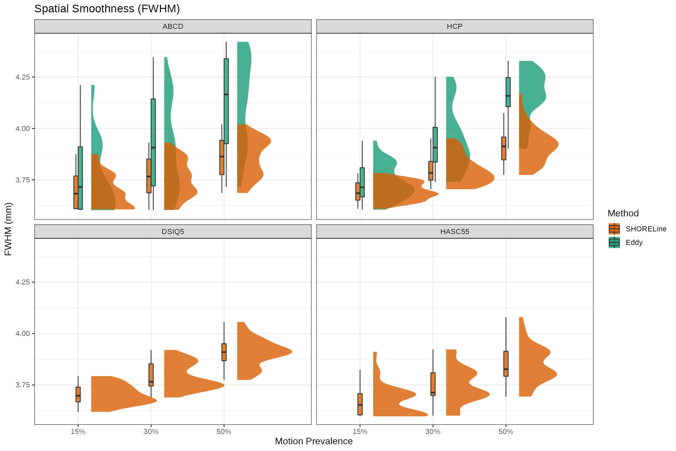

ggsave(here("vignettes","fwhm_smooth_plot.svg"),
       plot=fwhm_smooth_plot,
       height=3,
       width=7.9,
       units="in")

# What about if we make a paired comparison?
id_cols <- c("scheme", "iternum", "method", "denoising", "percent_motion")

paired_fwhm <- qc_df %>% 
  select(one_of(c(id_cols, "fwhm"))) %>%
  spread(method, fwhm, sep="_") %>%
  mutate(fwhm_diff=method_SHORELine - method_Eddy,
         percent_motion = as.factor(paste0(percent_motion, "%"))) %>%
  select(-starts_with("method_")) %>%
  
  # make it presentable for the table
  mutate(
    Denoising = denoising,
    Scheme = scheme,
    `Motion Prevalence` = percent_motion
  )
  
  
fwhm_diff_model <- lm(
  fwhm_diff ~ `Motion Prevalence` + Scheme + Denoising,
  data=paired_fwhm)

capt <- "**Supplementary Listing 3: Evaluating Smoothness of Preprocessed Data Following Head Motion Correction Quantified by FWHM.** The SHORELine FWHM value was subtracted from the Eddy FWHM, and this difference was the outcome variable of the model. Across all sampling schemes and method correction methods, more motion is associated with greater smoothness in output images. SHORELine produced significantly sharper outputs than Eddy."

tbl_regression(
  fwhm_diff_model,
  intercept=TRUE,
  estimate_fun = ~style_number(.x, digits=3)
  ) %>%
  bold_p() %>%
  bold_labels() %>% 
  italicize_levels() %>%
  as_gt() %>%
  tab_header(title = "Predicting FWHM (Eddy — Shoreline) of Each Scan",
             #subtitle = "Main Effects of Percent Motion, Scheme, and Denoising"
             ) %>%
  # tab_source_note(md(capt)) %>%
  # tab_style(
  #   style = cell_text(
  #     size = "large"
  #   ),
  #   locations = cells_source_notes()
  # ) %>% 
  opt_table_font("Helvetica") -> fwhm_model

fwhm_model

Predicting FWHM (Eddy — Shoreline) of Each Scan
Characteristic	Beta	95% CI¹	p-value
(Intercept)	-0.060	-0.083, -0.036	<0.001
Motion Prevalence
15%	—	—
30%	-0.086	-0.111, -0.060	<0.001
50%	-0.199	-0.225, -0.174	<0.001
Scheme
ABCD	—	—
HCP	0.018	-0.002, 0.039	0.084
Denoising
MP-PCA	—	—
None	-0.009	-0.030, 0.012	0.4
¹ CI = Confidence Interval

fwhm_model %>% gtsave(here("figures", "fwhm_model.pdf"), zoom=1)

3. Comparing FWHM-corrected NDC between SHORELine and Eddy

Does one of the methods have higher NDC scores? Also what is the improvement in NDC relative to the raw data? We know that higher percent motion will cause lower NDC scores in the unprocessed data.

improved_ndc_summaries <- qc_df %>%
  group_by(denoising, scheme, method, percent_motion) %>%
  summarise(mean_ndc=mean(improved.ndc.corrected), 
            sd_ndc=sd(improved.ndc.corrected), 
            se_ndc=sd_ndc/sqrt(length(improved.ndc.corrected)),
            group_mean_ndc=mean(mean_ndc),
            sd_mean_ndc=sd(mean_ndc))

## `summarise()` has grouped output by 'denoising', 'scheme', 'method'. You can
## override using the `.groups` argument.

improved_ndc_summaries$measure <- 'NDC Change\nFrom Raw'
ndc_summaries <- qc_df %>%
  group_by(denoising, scheme, method, percent_motion) %>%
  summarise(mean_ndc=mean(ndc.corrected), 
            sd_ndc=sd(ndc.corrected), 
            se_ndc=sd_ndc/sqrt(length(ndc.corrected)),
            group_mean_ndc=mean(mean_ndc),
            sd_mean_ndc=sd(mean_ndc))

## `summarise()` has grouped output by 'denoising', 'scheme', 'method'. You can
## override using the `.groups` argument.

ndc_summaries$measure <- 'Preprocessed NDC'
qc_summaries <- rbind(ndc_summaries, improved_ndc_summaries)
qc_summaries$percent_motion <- as.factor(qc_summaries$percent_motion)
qc_summaries$measure <- factor(qc_summaries$measure, levels=c('Preprocessed NDC', 'NDC Change\nFrom Raw'))

pd=position_dodge(width=0.6, preserve="single")
ndc_mean_plt <-  
  ggplot(
    qc_summaries %>% mutate(percent_motion=paste0(percent_motion, "%")),
    aes(
      y=group_mean_ndc, x=percent_motion, 
      fill=method, group=interaction(method, denoising))
    ) +
  geom_bar(aes(alpha=denoising), stat="identity", position=pd, width = 0.6) +
  geom_errorbar(
    aes(ymax=group_mean_ndc+sd_ndc, ymin=group_mean_ndc-sd_ndc,
        width=0.6),
    color = "black", position=pd
    ) +
  facet_grid(measure~scheme, scales="free") +
  scale_fill_manual(
    values=c("SHORELine"="#d95f02", "Eddy"="#1b9e77")
    ) +
  scale_alpha_manual(
    name="Denoising Strategy",
    values=c(1.0, 0.5)
    ) +
  theme_bw(
    base_family="Helvetica",
    base_size=12
  ) +
  theme(strip.text.y = element_text(size = 8)) +
  labs(title = "QC Measure", 
       y = "Neighboring DWI Correlation", 
       x = "Motion Prevalence",
       fill = "Method"
       ) +
  guides(linetype=guide_legend(override.aes=list(fill=NA)))

ndc_mean_plt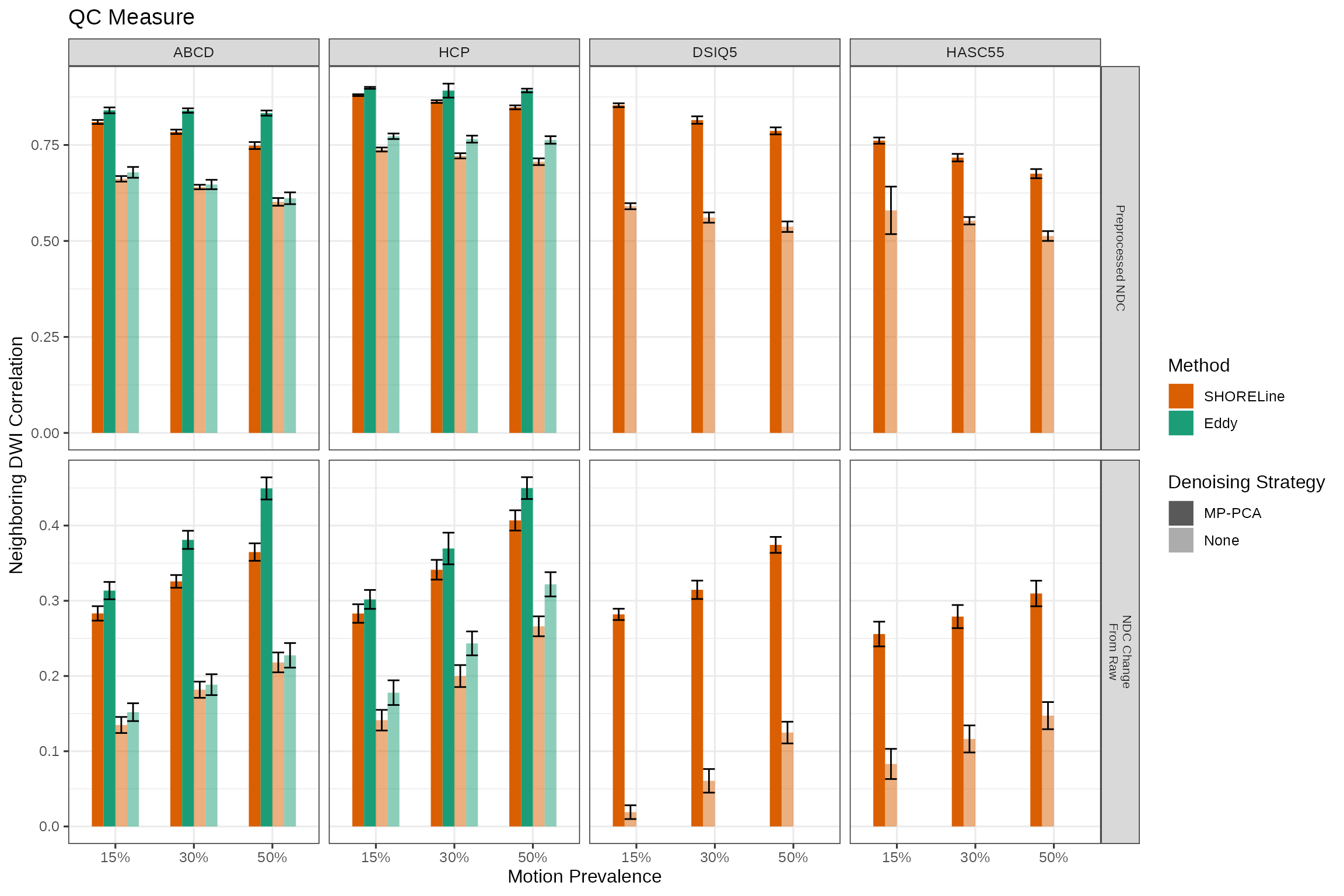

ggsave(here("vignettes","ndc_mean_plot.svg"),
       plot=ndc_mean_plt,
       height=3.5,
       width=7.9,
       units="in")

The NDC scores in and of themselves don’t mean much across sampling schemes, but are comparable within sampling schemes. The top row shows that MP-PCA improves NDC scores across the board and also that Eddy has a small advantage in the two shelled schemes where it can be used.

The second row shows the percent improvement in NDC relative to the raw scans. This is pretty remarkable. To do statistical tests, we will center the raw NDC within their percent motion category

qc_df <- subset(qc_df, scheme %in% c("ABCD", "HCP"))

ggplot(qc_df, aes(x=percent_motion, y=raw_neighbor_corr, color=scheme)) + 
  geom_jitter() +
  ggtitle("Unprocessed data NDC values")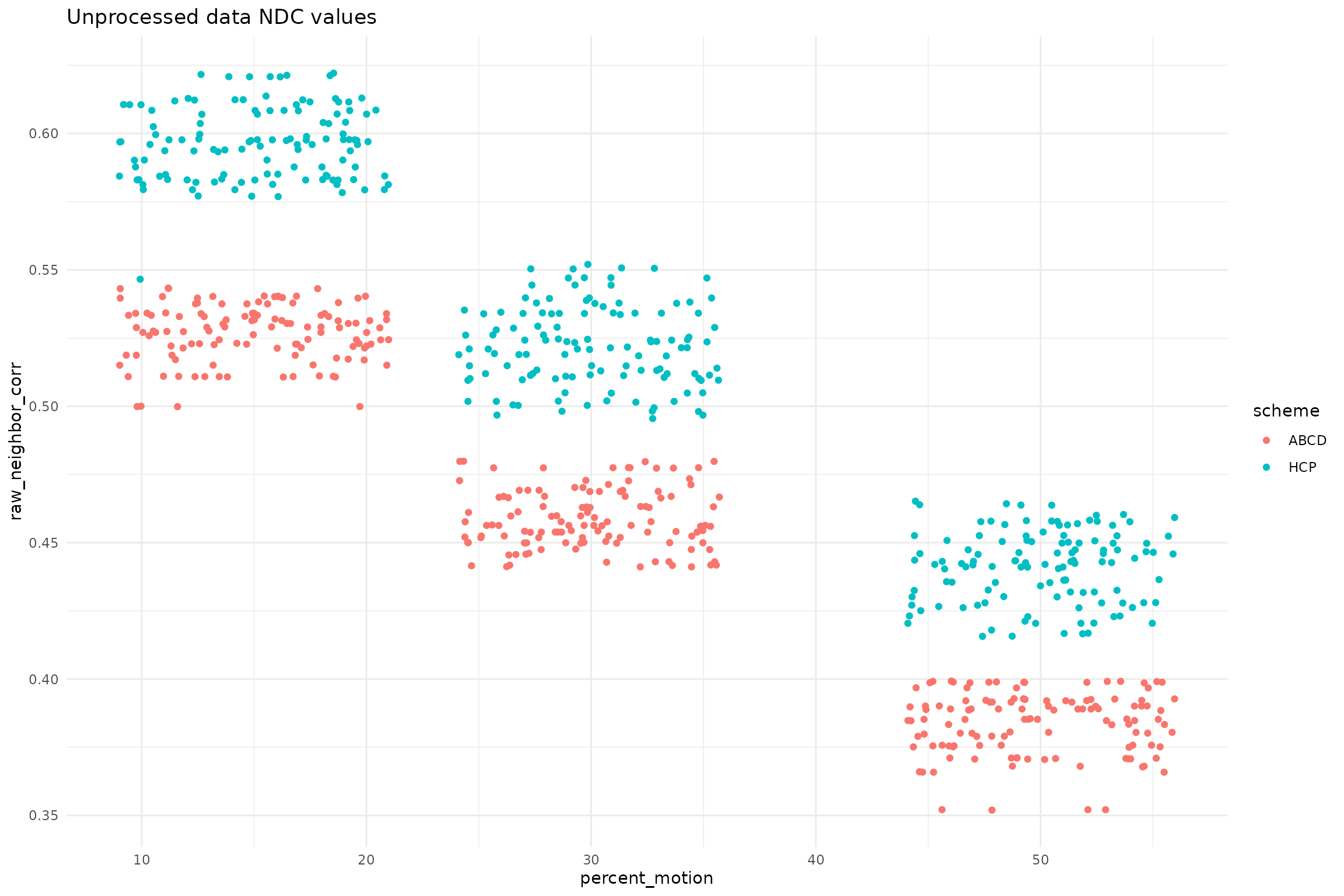

qc_df <- qc_df %>%
   group_by(percent_motion) %>%
   mutate(pct_motion_mean=median(raw_neighbor_corr),
          centered_raw_ndc=raw_neighbor_corr - pct_motion_mean)

ggplot(qc_df, aes(x=percent_motion, y=centered_raw_ndc, color=scheme)) + 
  geom_jitter() +
  ggtitle("Unprocessed data NDC values: Centered by percent motion")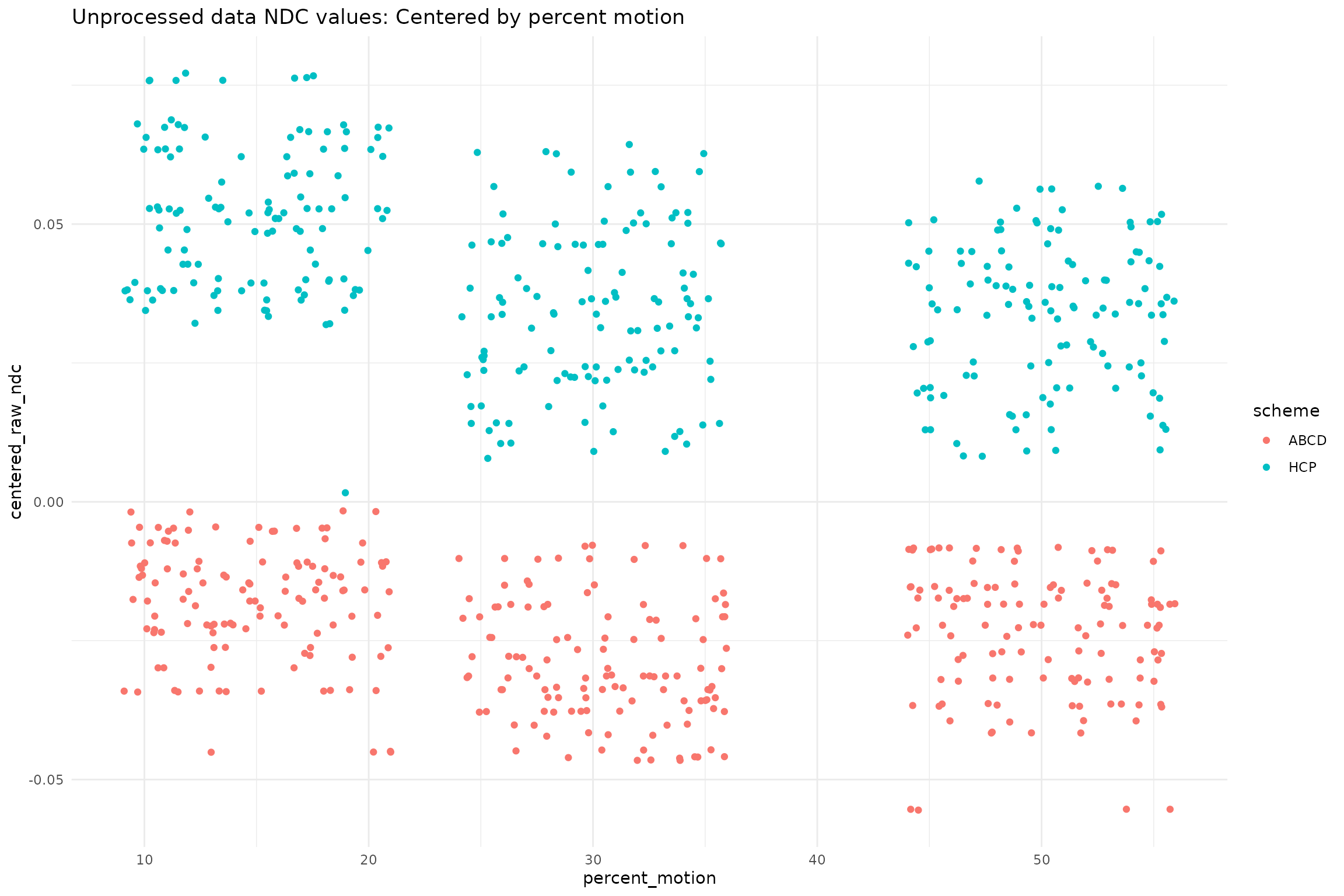

paired_ndc <- qc_df %>% 
  select(one_of(c(id_cols, "ndc.corrected"))) %>%
  spread(method, ndc.corrected, sep="_") %>%
  mutate(ndc_diff=method_SHORELine - method_Eddy) %>%
  select(-starts_with("method_")) %>%
    # make it presentable for the table
  mutate(
    Denoising = denoising,
    Scheme = scheme,
    `Motion Prevalence` = percent_motion
  )

ndc_diff_model <- lm(
  ndc_diff ~ `Motion Prevalence` + Denoising + Scheme,
  data=paired_ndc)

tbl_regression(
  ndc_diff_model,
  intercept=TRUE,
  estimate_fun = ~style_number(.x, digits=3)
  ) %>%
  bold_p() %>%
  bold_labels() %>% 
  italicize_levels() %>%
  as_gt() %>%
  tab_header(title = "NDC Model") %>%
  #tab_source_note(md("*This data is simulated*")) %>%
  opt_table_font("Helvetica") -> ndc_table

ndc_table

NDC Model
Characteristic	Beta	95% CI¹	p-value
(Intercept)	-0.020	-0.026, -0.014	<0.001
Motion Prevalence	-0.001	-0.001, -0.001	<0.001
Denoising
MP-PCA	—	—
None	0.016	0.011, 0.020	<0.001
Scheme
ABCD	—	—
HCP	-0.004	-0.008, 0.000	0.072
¹ CI = Confidence Interval

ndc_table %>% gtsave(here("figures", "ndc_model.pdf"), vwidth=250, vheight=100)

2022-07-20