---
title: "Classic vs TRX: A Complete Tractography Walkthrough"
subtitle: "HCP Data · Glasser 360 + Schaefer 4S456 · NODDI scalars · 500k streamlines"
execute:
echo: true
eval: true
warning: false
error: false
freeze: auto
---
```{r}
#| label: r-setup
#| include: false
# Working directory for all bash chunks — created here, used throughout
wd <- file.path(dirname(normalizePath(knitr::current_input())), "walkthrough")
dir.create(wd, showWarnings = FALSE)
knitr::opts_knit$set(root.dir = wd)
# Prepend trx-mrtrix build binaries and miniforge3 so bash chunks find them
Sys.setenv(PATH = paste0(
"/Users/mcieslak/projects/trx-mrtrix/build/bin",
":/Users/mcieslak/miniforge3/bin",
":", Sys.getenv("PATH")
))
# Number of streamlines — small for a fast demo render; scale up for production
Sys.setenv(N_TRACKS = "1000000")
```
::: {.callout-note}
## Rendering notes
This document executes during render (`eval: true`). All MRtrix binaries come
from the `trx-mrtrix` build at `build/bin/`, not the system installation.
The demo uses **1M streamlines** for a long render; change `N_TRACKS`
in the R setup chunk to make it faster/slower.
:::
## Timing and resource measurement
Every major command is wrapped with `mtime` — a thin shell function around
`/usr/bin/time -l` (macOS) that emits a one-line summary after each step:
```
┌─ tckgen (TRX)              ─────────────────────────────────────────────┐
│  wall:    52.3s    user:   812.4s    sys:    6.1s    peak mem: 2.31 GB  │
└─────────────────────────────────────────────────────────────────────────┘
```
| Metric | What it measures |
|--------|-----------------|
| **wall** | Elapsed clock time — the number you actually wait |
| **user** | Total CPU time across all threads; `user >> wall` for multithreaded commands |
| **sys** | Kernel time (I/O, memory mapping) |
| **peak mem** | Physical memory footprint (`phys_footprint` via `TASK_VM_INFO`) — excludes clean read-only mmap pages, so TRX files are not double-counted |
::: {.callout-note collapse="true"}
## Why not RSS?
`maximum resident set size` (RSS) counts clean file-backed mmap pages — TRX
files are opened read-only via mmap, so RSS is inflated for TRX inputs even
though those pages impose no memory pressure. **`peak memory footprint`**
counts only dirty/anonymous pages and matches what Activity Monitor shows.
:::
---
## Setup
```{bash}
#| label: setup
DERIV=/Users/mcieslak/data/qsirecon/derivatives/qsirecon-MRtrix3_act-HSVS/sub-100307/dwi
PARC=/Users/mcieslak/data/qsirecon/sub-100307/dwi

source ../timing_utils.sh

ln -sf "$DERIV/sub-100307_space-T1w_model-msmtcsd_param-fod_label-WM_dwimap.mif.gz" wm_fod.mif.gz
ln -sf "$DERIV/sub-100307_space-T1w_model-mtnorm_param-inliermask_dwimap.nii.gz"     mask.nii.gz
ln -sf "$PARC/sub-100307_space-T1w_model-noddi_param-icvf_dwimap.nii.gz"             icvf.nii.gz
ln -sf "$PARC/sub-100307_space-T1w_model-noddi_param-isovf_dwimap.nii.gz"            isovf.nii.gz
ln -sf "$PARC/sub-100307_space-T1w_seg-Glasser_dseg.mif.gz"                          glasser.mif.gz
ln -sf "$PARC/sub-100307_space-T1w_seg-Glasser_dseg.txt"                             glasser.txt
ln -sf "$PARC/sub-100307_space-T1w_seg-4S456Parcels_dseg.mif.gz"                     4S456.mif.gz
ln -sf "$PARC/sub-100307_space-T1w_seg-4S456Parcels_dseg.txt"                        4S456.txt

echo "N_TRACKS = $N_TRACKS"
echo "tckgen:   $(which tckgen)"
echo "trxlabel: $(which trxlabel)"
ls -lh *.mif.gz *.nii.gz *.txt
```
---
## Step 1 — Generate streamlines
Both pipelines start from a common `tckgen` run. MRtrix selects the writer
from the output filename extension, so the only difference is `.tck` vs `.trx`.
:::: {.columns}
::: {.column width="49%"}
<span class="badge-classic">CLASSIC</span>
```{bash}
#| label: tckgen-classic
source ../timing_utils.sh
mtime "tckgen (classic)" \
tckgen wm_fod.mif.gz       \
    -algorithm iFOD2        \
    -seed_image mask.nii.gz \
    -mask       mask.nii.gz \
    -minlength  30          \
    -maxlength  250         \
    -select     $N_TRACKS   \
    -nthreads   8           \
    -force                  \
    tracks.tck
```
```{bash}
tckinfo tracks.tck
du -sh  tracks.tck
```
:::
::: {.column width="49%"}
<span class="badge-trx">TRX</span>
```{bash}
#| label: tckgen-trx
source ../timing_utils.sh
mtime "tckgen (TRX float16)" \
tckgen wm_fod.mif.gz       \
    -algorithm iFOD2        \
    -seed_image mask.nii.gz \
    -mask       mask.nii.gz \
    -minlength  30          \
    -maxlength  250         \
    -select     $N_TRACKS   \
    -nthreads   8           \
    -trx_float16            \
    -force                  \
    tracks_f16.trx
```
```{bash}
tckinfo tracks_f16.trx
du -sh  tracks_f16.trx
```
:::
::::
The float16 TRX is roughly **half the size** of the TCK at the same streamline
count. For the remainder of this walkthrough we use `tckconvert` to produce a
float32 TRX from the same TCK, so both pipelines operate on **byte-for-byte
identical streamlines** and any output differences are purely due to format, not
stochastic variation.
```{bash}
#| label: tckconvert-trx
source ../timing_utils.sh
mtime "tckconvert → TRX" \
tckconvert tracks.tck tracks.trx -force
```
```{bash}
tckinfo tracks.trx
du -sh  tracks.trx
```
---
## Step 2 — SIFT2 weighting
SIFT2 calibrates per-streamline weights to match the WM FOD amplitudes. In the
classic pipeline the weights land in a separate CSV. In the TRX pipeline they
are embedded as a `data_per_streamline` field named `weights`.
:::: {.columns}
::: {.column width="49%"}
<span class="badge-classic">CLASSIC</span>
```{bash}
#| label: sift2-classic
source ../timing_utils.sh
mtime "tcksift2 (classic)" \
tcksift2                   \
    tracks.tck             \
    wm_fod.mif.gz          \
    weights_classic.csv    \
    -nthreads 8            \
    -force
```
```{bash}
wc -l weights_classic.csv
du -sh tracks.tck weights_classic.csv
```
:::
::: {.column width="49%"}
<span class="badge-trx">TRX</span>
```{bash}
#| label: sift2-trx
source ../timing_utils.sh
mtime "tcksift2 (TRX)" \
tcksift2               \
    tracks.trx         \
    wm_fod.mif.gz      \
    weights            \
    -nthreads 8        \
    -force
```
```{bash}
tckinfo tracks.trx
```
:::
::::
---
## Step 3 — Sample NODDI scalar maps
NODDI provides two microstructure metrics:
- **ICVF** (intracellular volume fraction) — neurite density proxy
- **ISOVF** (isotropic volume fraction) — free water content
`tcksample` interpolates a volumetric image at every streamline vertex, yielding:
- **dpv** (per-vertex) — full sampled profile; used for mrview coloring and along-tract statistics
- **dps mean** (per-streamline) — one number per streamline; useful as a connectivity weight or covariate
:::: {.columns}
::: {.column width="49%"}
<span class="badge-classic">CLASSIC</span>
```{bash}
#| label: tcksample-classic
source ../timing_utils.sh
mtime "tcksample icvf dpv" \
tcksample tracks.tck icvf.nii.gz icvf.tsf -force

mtime "tcksample isovf dpv" \
tcksample tracks.tck isovf.nii.gz isovf.tsf -force

mtime "tcksample icvf mean" \
tcksample tracks.tck icvf.nii.gz icvf_mean.txt -stat_tck mean -force

mtime "tcksample isovf mean" \
tcksample tracks.tck isovf.nii.gz isovf_mean.txt -stat_tck mean -force

du -sh icvf.tsf isovf.tsf icvf_mean.txt isovf_mean.txt
```
:::
::: {.column width="49%"}
<span class="badge-trx">TRX</span>
```{bash}
#| label: tcksample-trx
source ../timing_utils.sh
mtime "tcksample icvf dpv" \
tcksample tracks.trx icvf.nii.gz icvf

mtime "tcksample isovf dpv" \
tcksample tracks.trx isovf.nii.gz isovf

mtime "tcksample icvf mean" \
tcksample tracks.trx icvf.nii.gz icvf_mean -stat_tck mean

mtime "tcksample isovf mean" \
tcksample tracks.trx isovf.nii.gz isovf_mean -stat_tck mean

tckinfo -prefix_depth 2 tracks.trx
```
:::
::::
---
## Step 4 — Visualize results in mrview
`mrview` loads TRX files directly. The SIFT2 weights and NODDI scalars embedded
in the previous two steps are immediately available as colormap sources — no
sidecar files to locate or load separately.
Open `tracks.trx` in `mrview → Tools → Tractography → Colour → Scalar file → TRX field…`
and select `icvf`, `isovf`, or `weights` for per-vertex or per-streamline coloring.
If a field name exists in both dps and dpv, disambiguate using `dps:<name>` or `dpv:<name>`.
Command-line capture via `-capture.folder`, `-capture.prefix`, and `-capture.grab`
works with TRX inputs (requires a live GUI session):
```{bash}
mrview mask.nii.gz \
  -mode 2 \
  -imagevisible 0 \
  -tractography.load tracks.trx \
  -tractography.geometry lines \
  -tractography.opacity 1.0 \
  -tractography.thickness 0.25 \
  -tractography.slab -1 \
  -tractography.trx_scalar dps:weights \
  -tractography.tsf_range 0.15,2.5 \
  -capture.folder . \
  -capture.prefix trx_sift_overlay \
  -capture.grab \
  -exit
```
```{bash}
#| label: mrview-capture-and-embed
#| results: asis
source ../timing_utils.sh
rm -f trx_sift_overlay*.png mrview_trx_overlay.png mrview_trx_overlay_fallback.svg
rm -f ../mrview_trx_overlay.png ../mrview_trx_overlay_fallback.svg
set +e
mrview mask.nii.gz \
-mode 2 \
-imagevisible 0 \
-tractography.load tracks.trx \
-tractography.geometry lines \
-tractography.opacity 1.0 \
-tractography.thickness 0.25 \
-tractography.slab -1 \
-tractography.trx_scalar dps:weights \
-tractography.tsf_range 0.15,2.5 \
-capture.folder . \
-capture.prefix trx_sift_overlay \
-capture.grab \
-exit
mrview_status=$?
set -e
capture_file=""
for f in trx_sift_overlay*.png; do
if [ -f "$f" ]; then
capture_file="$f"
break
fi
done
if [ -n "$capture_file" ]; then
cp "$capture_file" mrview_trx_overlay.png
cp "$capture_file" ../mrview_trx_overlay.png
echo "Captured mrview image: \`$capture_file\`"
echo ""
echo "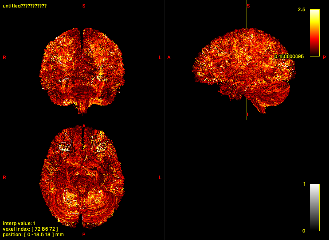"
fi
```
---
## Step 5 — Atlas labeling and connectome construction
`tck2connectome` assigns streamlines to node pairs on-the-fly — the assignment
is ephemeral and must be recomputed for every new atlas or metric.
`trxlabel` embeds the assignment as TRX groups permanently. Multiple atlases
can be labeled in a **single pass** over the tractogram by repeating `-nodes`,
`-lut`, and `-prefix` — geometry is read exactly once regardless of how many
atlases are requested.
### 4a — Classic: two separate tck2connectome runs
The classic pipeline must reread all geometry and redo the radial search for each atlas.
```{bash}
#| label: tck2connectome-glasser-classic
source ../timing_utils.sh
mtime "tck2connectome Glasser" \
tck2connectome                  \
    tracks.tck                  \
    glasser.mif.gz              \
    connectome_glasser_classic.csv \
    -tck_weights_in weights_classic.csv \
    -assignment_radial_search 2 \
    -symmetric                  \
    -zero_diagonal              \
    -force
```
```{bash}
#| label: tck2connectome-4S456-classic
source ../timing_utils.sh
mtime "tck2connectome 4S456" \
tck2connectome                  \
    tracks.tck                  \
    4S456.mif.gz                \
    connectome_4S456_classic.csv \
    -tck_weights_in weights_classic.csv \
    -assignment_radial_search 2 \
    -symmetric                  \
    -zero_diagonal              \
    -force
```
### 4b — TRX: both atlases in a single trxlabel pass
`trxlabel` accepts multiple `-nodes`/`-lut`/`-prefix` triplets and labels all
atlases in one pass over the tractogram — no geometry is read twice.
```{bash}
#| label: trxlabel-both
source ../timing_utils.sh
mtime "trxlabel Glasser + 4S456" \
trxlabel                         \
    tracks.trx tracks.trx        \
    -nodes  glasser.mif.gz       \
    -nodes  4S456.mif.gz         \
    -lut    glasser.txt          \
    -lut    4S456.txt            \
    -prefix glasser              \
    -prefix 4S456                \
    -assignment_radial_search 2  \
    -force
```
```{bash}
#| label: tckinfo-after-label
tckinfo -prefix_depth 2 tracks.trx
```
```{bash}
#| label: trx2connectome-glasser
source ../timing_utils.sh
mtime "trx2connectome Glasser" \
trx2connectome                   \
    tracks.trx                   \
    connectome_glasser_trx.csv   \
    -tck_weights_in weights      \
    -out_node_names glasser_nodes.txt \
    -group_prefix glasser        \
    -lut glasser.txt             \
    -symmetric                   \
    -zero_diagonal               \
    -force
```
```{bash}
#| label: trx2connectome-4S456
source ../timing_utils.sh
mtime "trx2connectome 4S456" \
trx2connectome                 \
    tracks.trx                 \
    connectome_4S456_trx.csv   \
    -tck_weights_in weights    \
    -out_node_names 4S456_nodes.txt \
    -group_prefix 4S456        \
    -lut 4S456.txt             \
    -symmetric                 \
    -zero_diagonal             \
    -force
```
```{bash}
#| label: tckinfo-final
tckinfo -prefix_depth 2 tracks.trx
```
### 4c — TRX combined-atlas connectome in one matrix
Because both atlas group sets are embedded in one TRX file, `trx2connectome`
can emit a single matrix that includes:
- within-atlas edges (Glasser-Glasser, 4S456-4S456), and
- cross-atlas edges (Glasser-4S456),
without rerunning any node assignment.
```{bash}
#| label: trx2connectome-combined
source ../timing_utils.sh
mtime "trx2connectome combined-atlas matrix" \
trx2connectome \
    tracks.trx \
    connectome_combined_trx.csv \
    -tck_weights_in weights \
    -out_node_names combined_nodes.txt \
    -symmetric \
    -zero_diagonal \
    -force
```
```{bash}
#| label: combined-connectome-summary
python3 - <<'EOF'
import collections
import itertools
import numpy as np

mat = np.loadtxt("connectome_combined_trx.csv", delimiter=",")
names = [line.strip() for line in open("combined_nodes.txt") if line.strip()]

def atlas_prefix(name: str) -> str:
    return name.split("_", 1)[0] if "_" in name else "(no_prefix)"

if mat.shape[0] != len(names):
    raise RuntimeError(f"matrix shape {mat.shape} does not match node-name list length {len(names)}")

prefix_counts = collections.Counter(atlas_prefix(n) for n in names)
print(f"combined matrix shape: {mat.shape}")
print("node counts by atlas prefix:")
for k in sorted(prefix_counts):
    print(f"  {k}: {prefix_counts[k]}")

indices = {k: [i for i, n in enumerate(names) if atlas_prefix(n) == k] for k in sorted(prefix_counts)}
print("non-zero edge counts by atlas block:")
for a, b in itertools.combinations_with_replacement(sorted(indices), 2):
    block = mat[np.ix_(indices[a], indices[b])]
    nnz = int((block > 0).sum())
    total = float(block.sum())
    print(f"  {a:>8s} x {b:<8s}: nnz={nnz:6d}, sum={total:.3f}")
EOF
```
---
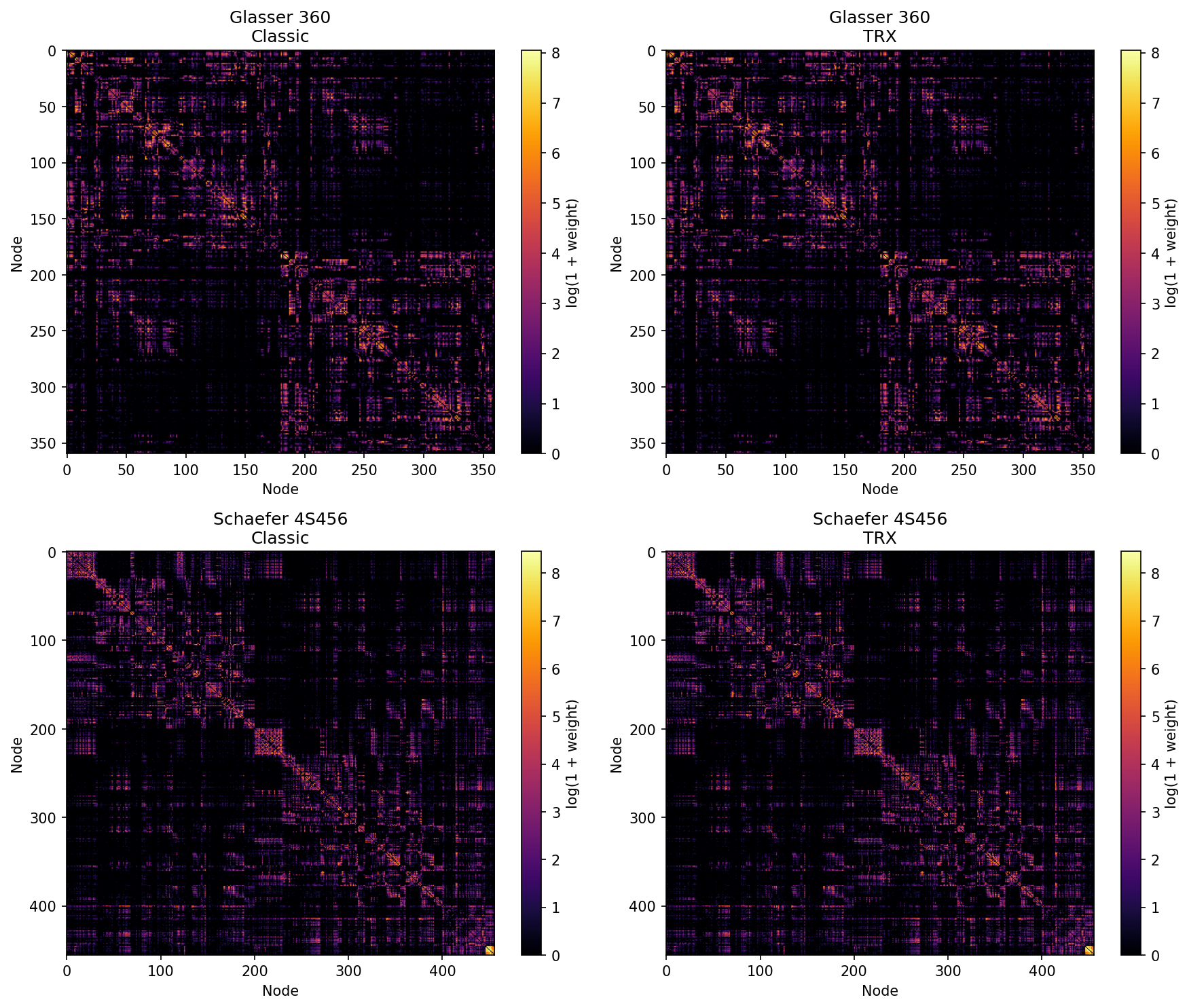
## Step 6 — Verify equivalence
With `-lut`, `trx2connectome` orders rows and columns by numeric node ID —
the same ordering `tck2connectome` uses. The matrices are directly comparable
with no reordering.
```{bash}
#| label: diff-connectomes
python3 - <<'EOF'
import numpy as np, sys
ok = True
for atlas in [("Glasser", "connectome_glasser_classic.csv", "connectome_glasser_trx.csv"),
              ("4S456",   "connectome_4S456_classic.csv",   "connectome_4S456_trx.csv")]:
    name, cf, tf = atlas
    a = np.loadtxt(cf, delimiter=",")
    b = np.loadtxt(tf, delimiter=",")
    if a.shape != b.shape:
        print(f"{name}: SHAPE MISMATCH  classic={a.shape}  trx={b.shape}", file=sys.stderr)
        ok = False
        continue
    diff = np.abs(a - b)
    print(f"{name} {a.shape}  max|diff|={diff.max():.2e}  mean|diff|={diff.mean():.2e}")
    if diff.max() > 0.5:
        ok = False
        print(f"  FAIL: differences too large", file=sys.stderr)
if ok:
    print("All matrices match (within rounding).")
else:
    sys.exit(1)
EOF
```
```{bash}
#| label: heatmaps
python3 - <<'EOF'
import numpy as np
import matplotlib
matplotlib.use("Agg")
import matplotlib.pyplot as plt

pairs = [
    ("Glasser 360",    "connectome_glasser_classic.csv", "connectome_glasser_trx.csv"),
    ("Schaefer 4S456", "connectome_4S456_classic.csv",   "connectome_4S456_trx.csv"),
]

fig, axes = plt.subplots(2, 2, figsize=(12, 10))
for row, (name, cf, tf) in enumerate(pairs):
    classic = np.loadtxt(cf, delimiter=",")
    trx     = np.loadtxt(tf, delimiter=",")
    for col, (mat, title) in enumerate([(classic, f"{name}\nClassic"), (trx, f"{name}\nTRX")]):
        ax = axes[row][col]
        im = ax.imshow(np.log1p(mat), cmap="inferno", aspect="auto")
        ax.set_title(title)
        ax.set_xlabel("Node")
        ax.set_ylabel("Node")
        plt.colorbar(im, ax=ax, label="log(1 + weight)")

plt.tight_layout()
plt.savefig("../connectome_comparison.png", dpi=150, bbox_inches="tight")
print("Saved connectome_comparison.png")
EOF
```
---
## Step 7 — File inventory
```{bash}
#| label: file-inventory
echo "=== Classic: files required to reproduce either connectome ==="
ls -lh tracks.tck weights_classic.csv icvf.tsf isovf.tsf icvf_mean.txt isovf_mean.txt \
        connectome_glasser_classic.csv connectome_4S456_classic.csv

echo ""
echo "=== TRX: everything in one file ==="
ls -lh tracks.trx connectome_glasser_trx.csv connectome_4S456_trx.csv
```
---
## What's next
::: {.callout-tip}
### Other commands that read/write TRX fields
| Command | TRX capability |
|---------|---------------|
| `tckedit` | Filters TRX by ROI, length, or count; remaps dps/dpv/groups to surviving streamlines |
| `tcksift` | Produces a TRX subset via `subset_streamlines` — all metadata preserved |
| `fixel2tsf` | Pass a bare field name as output to embed fixel scalars as dpv directly in TRX |
| `tsfinfo` / `tsfvalidate` | Inspect and validate TRX dpv fields |
| `mrview` | Loads TRX directly; colour by group, dps, or dpv field from the GUI |
:::

