Linking Individual Differences in Personalized Functional Network Topography to Psychopathology in Youth

Abstract: The spatial distribution of personalized large-scale functional networks on the association cortex develops in youth and is associated with executive function. However, it remains unknown if this personalized functional topography is related to the psychopathology. Capitalizing on a large sample imaged with 27 min of high-quality functional MRI data (n = 790, ages 8-23 years), we examined the relationship between personalized functional network topography and four correlated psychopathology dimensions as well as the overall psychopathology factor, which reflects a shared vulnerability to a broad range of symptoms across mental disorders. We found that the functional topography significantly predicted individual differences in overall psychopathology factor, which underlies the association between functional topography and correlated dimensions of psychopathology. Interestingly, there was a negative association between the total cortical representation of association networks and factor scores of psychopathology dimensions. Our results emphasize the importance of considering functional neuroanatomy for personalized therapeutics.

Project Lead

Zaixu Cui

Faculty Leads

Theodore D. Satterthwaite

Analytic Replicator

Adam R. Pines

Collaborators

Adam R. Pines, Bart Larsen, Valerie J. Sydnor, Hongming Li, Azeez Adebimpe, Aaron F. Alexander-Bloch, Dani S. Bassett, Max Bertolero, Monica E. Calkins, Christos Davatzikos, Damien A. Fair, Ruben C. Gur, Raquel E. Gur, Tyler M. Moore, Sheila Shanmugan, Russell T. Shinohara, Jacob W. Vogel,Cedric H. Xia,Yong Fan

Current Project Status

In submission.

Datasets

PNC dataset:https://www.ncbi.nlm.nih.gov/projects/gap/cgi-bin/study.cgi?study_id=phs000607.v3.p2

Github Repository

https://github.com/PennLINC/pncsinglefuncparcel_psychopathology

Path to Data on Filesystem

/cbica/projects/pncSingleFuncParcel/pncSingleFuncParcel_psycho

CODE DOCUMENTATION

The steps below detail how to replicate all aspects of this project, from neuroimage processing to statistical anlysis and figure generation.

Step_1st_PrepareData

1. Step_1st_SubjectFilter.R:

   Select our sample (i.e., 790 subjects). Inclusion criteria: healthExcludev2 = 0; fsFinalExclude = 0; restExclude = 0; restExcludeVoxelwise = 0; nbackFcExclude = 0; nbackFcExcludeVoxelwise = 0; idemoFcExclude = 0; idemoFcExcludeVoxelwise = 0. Finally, a sample of 790 subjects was created.

2. Step_2nd_ExtractBehavior.R

   Extract correlated dimensions, bifactors, and item-level symptom of psychopathology.

3. Step_3rd_CopyStructFSFiles.R, Step_4th_DataFSProcessing.m, Step_5th_MergeModalities.m:

   Project fmri data into surface and then combine the three modalities.

4. Step_6th_tSNRMask_*:

   Generate the tSNR mask.

5. Step_7th_EFA.R, Step_8th_CFA:

   Plot figures for exploratory factor analysis (Figure 2) and confirmatory factor analysis (Figure 5).

6. Step_9th_Prevelance.R:

   Calculate the prevelance of disorders.

Step_2nd_SingleParcellation

Step1 to step4 are codes for single functional parcellation (Li et al., 2017, NeuroImage). See (https://github.com/hmlicas/Collaborative_Brain_Decomposition) for the toolbox of single parcellation.

1. Step_1st_CreatePrepData.m:

   Generate the spatial neighborhood for fsaverage5 surface space. After removing medial wall, we have 18715 vertices.

2. Step_2nd_ParcellationInitialize.m:

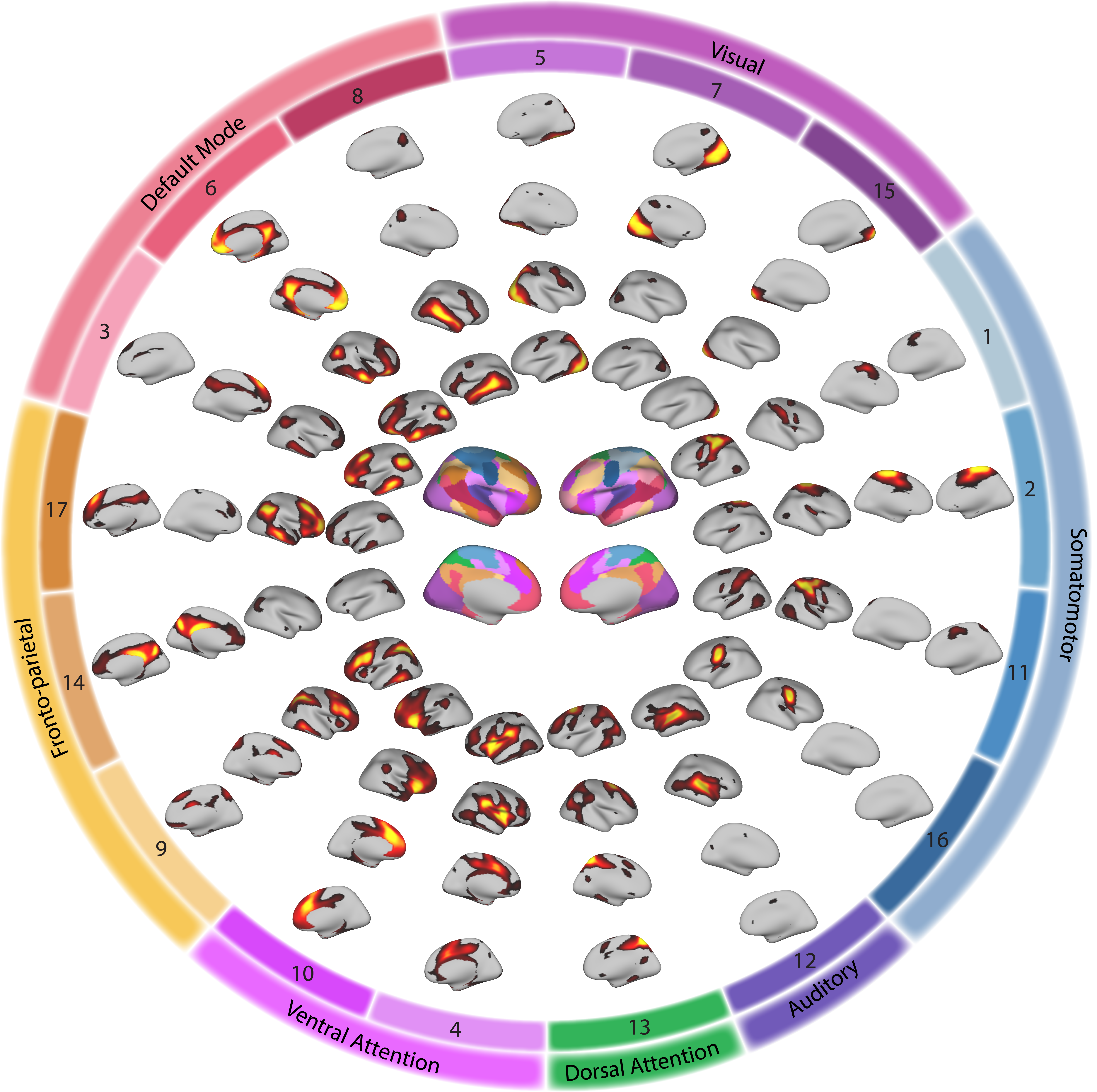
   Calculate the group parcellation, which will be the initialization of single subject parcellation. We randomly chose 100 subjects and combined these subjects’ data along time points and run non-negative matrix factorization (NMF) to decompose the whole brain into 17 networks. We repeated this procedure 50 times, finally 50 group atlas was acquired.

3. Step_3rd_SelRobustInit.m:

   Use normalized cuts based spectrum clustering method to cluster the acquired 50 group atlases. Finally, one group atlas with 17 networks was acquired.

4. Step_4th_IndividualParcel.m:

   Based on the acquired group atlas and the subject’s specific fMRI data, we calculated the atlas for this specific subject. Finally, each subject had a loading matrix, in which the loading value quantifies the probability each vertex belonging to each network.

5. Step_5th_AtlasInformation_Extract.m:

   Extract all subjects’ loading matrix information into the same folder. Also, extracting the discrete atlas for each subject by categorizing each vertex to the network with the highest loading, and put them into the same folder.

6. Step_6th_GroupAtlas_Extract.m:

   Extract loading matrix group atlas (the output of the script ‘Step_3rd_SelRobustInit.m’) and create the group discrete atlas by categorizing each vertex to the network with the highest loading.

7. Step_7th_NetworkNaming_Yeo.m:

   Calculate the overlap between our networks with Yeo atlas.

8. Step_8th_Visualize_Workbench_Atlas.m:

   Calculate inter-subjects variability of network loadings for each network using median absolute deviation and then average the 17 brain maps of variability.

9. Step_9th_Visualize_Workbench_AtlasVariability.m:

   Visualize the atlas variability map using workbench.

10. Step_10th_ViolinPlot_AtlasVariability_Loading.R:

    Visualize the variability of each network using violin plot.

Step_3rd_Psychopathology_SaveMat.R

Saving age, sex, motion, four correlated dimensions of psychopathology, five bifactors of psychopathology, and 112 item-level psychopathology symptoms to .mat file.

Step_4th_AtlasFeature_SaveMat.m

For each participant, extracting all the loadings of the 17 networks to be a high-dimensional feature vector.

Step_5th_PLSr1_Corrtraits

Prediction of the four correlated dimensions of psychopathology using personalized functional topography.

1. Step_1st_Prediction_*_RandomCV.py:

   Predict factor scores of fear, psychosis, externalizing and mood/anxious-misery dimensions using networks loading features acquired in Step 4th. Repeated (i.e., 101 times) two-fold cross validation (2F-CV) was used here. Partial least square regression was used to predict the behavior. We applied permutation testing (i.e., 1,000 times) to evaluate the significance of the prediction accuracy.

2. Step_2nd_Sig.m:

   Extract the prediction results and calculate the P value of the prediction accuracy based on the distribution from the permutation testing.

3. Step_3rd_Scatter_*.R:

   Plot the scatter plot of the correlation between actual and predicted scores of the prediction of the four correlated dimensions of psychopathology. The 2F-CV was repeated 101 times and we reported the one with the median prediction accuracy.

4. Step_4th_Permutation_All_Violin.R:

   Plot the actual prediction accuracy (i.e., correlation r between actual and predicted scores) and boxplot/violin plot of the permutation distribution.

5. Step_5th_Weight_Visualize_Workbench_*_RandomCV.m:

   Visualize the contribution pattern using workbench.

6. Step_6th_SumofWeights_*.R:

   Calculate the sum of weights within each of 17 networks and visualize using bar plot.

7. Step_7th_SumofWeights_Correlation.R:

   Calculate the correlation between the sum of weights and the median network variability, and then visualizing using scatter plot.

8. Step_8th_WeightsCorr_Plot.R & Step_9th_ContributionWeight_SpinTest:

   Calculate the correlation among the weight maps of the four dimensions and then test the significance using spin test

Step_6th_PLSr1_OverallPsyFactor

Prediction of overall psychopathology factor, which was from the bifactor model, using personalized functional topography. The computations from step 1 to step 6 are the same as the descriptions above. Particularly, Step 7th is testing the correlation between contribution maps and first gradient of functional hierarchy and evaluate the significance using spin test.

Step_7th_PLSr1_OtherFactors

Prediction of other specific orthogonal factors from bifactor model, including fear, psychosis, externalizing, mood/anxious-misery factors. Results showed functional topography significantly predicted fear and psychosis factors, so futher visualized the results of these two factors. The computations from step 1 and step 6 are the same with the above.

Step_8th_PLSca

Relate the functional topography and item-level psychopathology symptoms using partial least square correlation.

1. Step_1st_PLSCorr.py:

   Use partial least square correlation to decompose paris of components that maximizing the covariance between functional topography and item-level psychopathology symptoms. Repeated (i.e., 101 times) 2F-CV was used and a permutation testing was used to generate the distribution of out-of-sample correlations at chance level.

2. Step_2nd_PLSca_Sig.m:

   Extract the PLSC results and calculate the P value of the out-of-sample correlation between pairs of components.

3. Step_3rd_CovarianceExplained.R:

   Calculate the median covariance explained by each component across the 101 repetitions.

4. Step_4th_Scatter_PLSca.R:

   The scatter plot of the correlation between the first pair of components.

5. Step_5th_Prediction_RandomCV_All_Violin.R:

   The plot of the distribution of correlations between first pair of components from permutation testing.

6. Step_6th_BehaviorBrainFeatures_Update.m:

   Match the signs of weights across the 101 repetitions and calculate the P value of the contribution of each psychopathology item to the first component.

7. Step_7th_BrainFeatures.m:

   Visualize the contribution pattern of functional topography features to the first component.

8. Step_8th_SumofWeights_PLSca.R:

   Sum the contribution weights of each network and visualize using bar graph.

9. Step_9th_ContributionWeight_SpinTest:

   Evaluate the correlation between contribution maps of overall psychopathology factor from PLS-R and that from PLS-C and test the significance using permutation testing.

Notes

1. g_ls.m is a funtion that will be used in the Maltab scripts here. PSOM (http://psom.simexp-lab.org/) is used for parallelization. Both g_ls.m and PSOM can also be found in our previous software PANDA (https://github.com/ZaixuCui/PANDA; https://www.nitrc.org/projects/panda).
2. The folder “Functions” include the functions of fMRI data projection to surface, modalities merge, PLS regression and PLS correlation.