Cloud TileDB: RBC Cortical Thickness from S3

The Reproducible Brain Charts (RBC) FreeSurferPost release is available as a TileDB store on a public S3 bucket: 70 surface measures, each 327,684 fsLR-164k vertices by 8,696 sessions from five studies (BHRC, CCNP, HBN, NKI, PNC; ages 5–85). That is 553 GB. This article is about a report you can run yourself that fits models to those data without downloading them: ModelArray reads the handful of tiles it needs, straight from S3, and leaves the rest where it is.

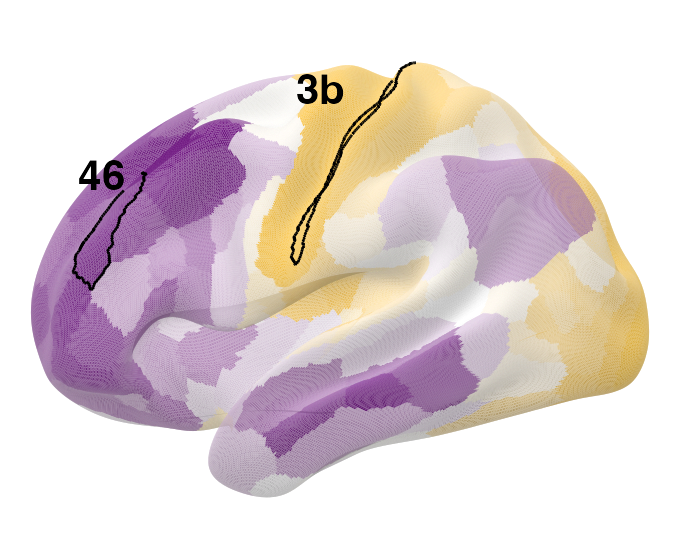
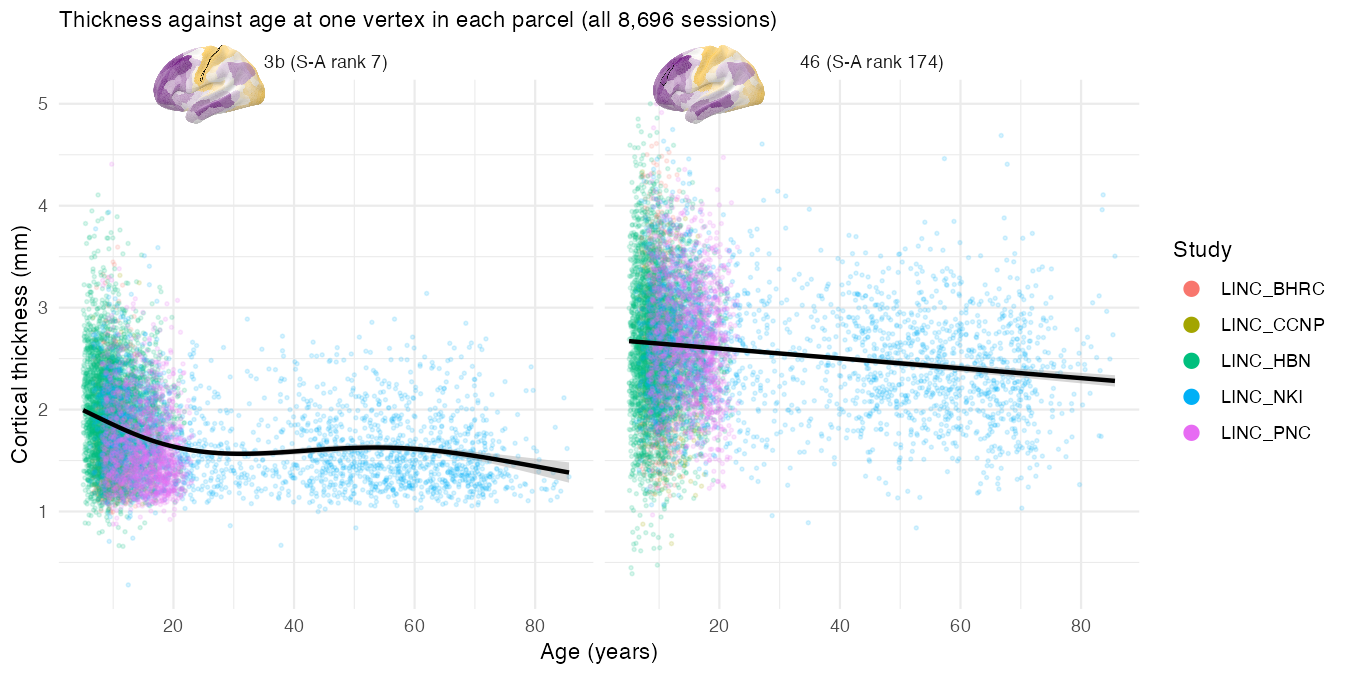
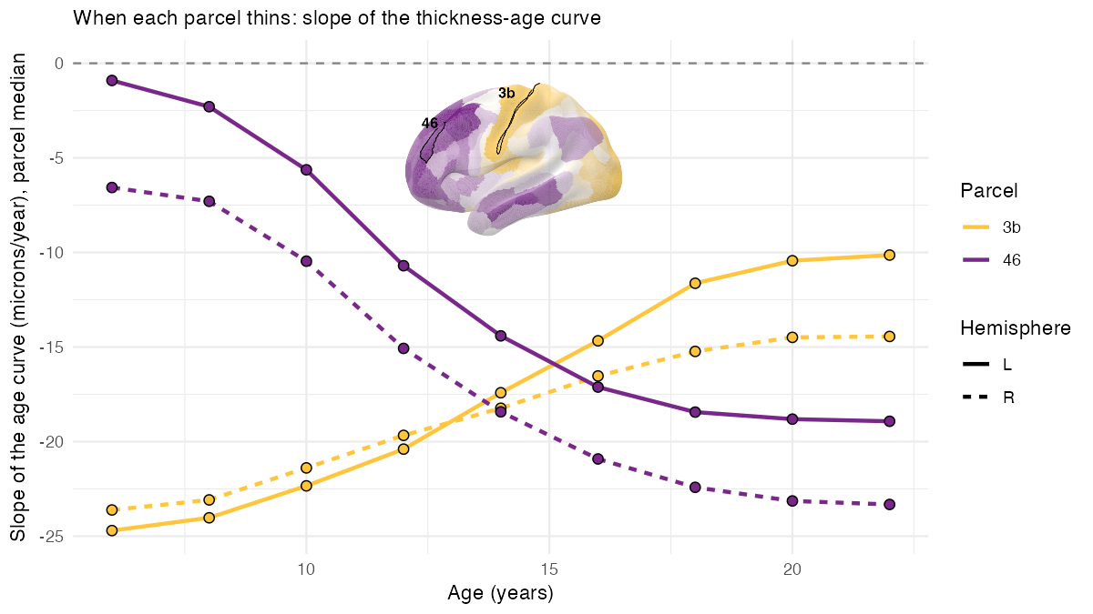
The report asks a question with a known answer, so you can tell whether it worked. The cortex thins through childhood and adolescence, but not everywhere at the same time: primary sensory cortex matures first and has little thinning left after mid-adolescence, while association cortex keeps thinning through the teens and into the twenties (Shaw et al., 2008; Tamnes et al., 2017). Sydnor et al. (2021) order every region along a sensorimotor–association (S-A) axis, from sensory and motor cortex at one end to prefrontal association cortex at the other. Put together: a parcel near the sensorimotor end should do most of its thinning early, and one near the association end should do most of it late. The report tests this on two Glasser parcels at opposite ends of the axis — area 3b (primary somatosensory, rank 7) and area 46 (dorsolateral prefrontal, rank 174) — one vertex at a time, and never on the whole cortex.

What the report does

Points TileDB at the bucket (two config settings, no AWS account).
Lists the store with ModelArraySummary(), opens thickness with ModelArray(), and downloads the cohort CSV (age, sex, site).
Works out, before reading anything, how many tiles each parcel touches and how many megabytes that is.
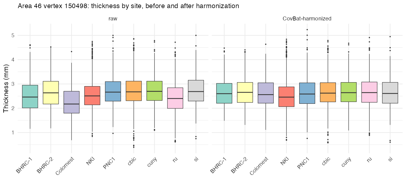
Looks at single vertices with exampleElementData(): thickness against age, a GAM with site as a covariate, its derivative, and a mixed model for repeat sessions.
Reads each parcel’s vertices from S3 in one go and harmonizes them across the nine scanning sites with CovBat (ComBatFamily::covfam(), keeping s(Age, k = 4) + sex), then writes the raw and harmonized blocks into a small local ModelArray store.
Runs ModelArray.gam() straight from S3 on one parcel (site as a covariate) and on the local store for every parcel, raw and harmonized, to show what harmonization changes; then ModelArray.wrap() with a custom fit_vertex() that adds an fx = TRUE test statistic, ΔR²adj, predicted thickness every two years and the derivative of the age curve with a simultaneous interval, for ages 5–23.
Summarizes per parcel, plots the late fraction of thinning and the slope-by-age curves against S-A rank, and compares them with the literature.
Writes CSVs, saves the results into the local store with writeResults(), and exports CIFTI dscalars plus .spec files for Connectome Workbench.
Prints how long each step took and how many bytes came over the wire.

Run it

In the browser

Click the Binder badge at the top. After a minute or two RStudio opens with ~/rbc_s3_example/rbc_s3_tiledb_example.Rmd ready; open it and press Knit. Binder gives one core and about 2 GB of memory, so the report detects it and uses its smallest settings (three left-hemisphere parcels, one tile each). Expect 10–15 minutes. Binder sessions are public and disappear after ten idle minutes, so download anything you want to keep (the rbc_s3_example folder has the HTML, CSVs and CIFTI files).

On your own machine

You need ModelArray from the GitHub main branch (TileDB support), the TileDB packages, and a few modelling packages:

install.packages(c("tiledb", "jsonlite", "mgcv", "ggplot2", "gratia", "gamm4", "lme4", "rmarkdown", "cowplot", "png"))
BiocManager::install("TileDBArray")
remotes::install_github("andy1764/ComBatFamily")
remotes::install_github("PennLINC/ModelArray")

Connectome Workbench is optional; with wb_command on your PATH the report writes the CIFTI files and a .spec you can open in wb_view. Then render:

example <- system.file("examples/rbc-s3-tiledb/rbc_s3_tiledb_example.Rmd", package = "ModelArray")
out_dir <- path.expand("~/rbc_s3_example")
dir.create(out_dir, recursive = TRUE, showWarnings = FALSE)

# quick: areas 3b and 46 in the left hemisphere, two tiles per parcel
rmarkdown::render(example, output_dir = out_dir, knit_root_dir = out_dir, intermediates_dir = tempdir(),
                  params = list(quick = TRUE, n_cores = 4, out_dir = out_dir))

# full: areas 3b and 46 in both hemispheres, six tiles per parcel
rmarkdown::render(example, output_dir = out_dir, knit_root_dir = out_dir, intermediates_dir = tempdir(),
                  params = list(quick = FALSE, n_cores = 8, out_dir = out_dir))

Other parameters (parcels, hemispheres, max_tiles_per_parcel, max_vertices_per_parcel, harmonize, write_cifti, allocation_mb) are listed at the top of the Rmd. The report never writes to S3; everything lands in out_dir.

What to expect

Numbers from runs on an Apple-silicon Mac (14 cores, 36 GB; the report used 8 cores).

	Quick	Full
Parcels	3b, 46 (left)	3b, 46 (both hemispheres)
Vertices analysed	600	2,000
Read from S3	296 MB (2 tiles per parcel)	996 MB (6 tiles per parcel)
CovBat	2.5 min on 2 cores	4.1 min on 4 cores
`fit_vertex()` at every vertex	42 s	3.6 min
Whole report	8 min	20 min

The full thickness scalar is 10.6 GB and the whole store 553 GB, so the full run reads about 0.2% of the store.

Every tile check passed: each parcel read exactly the tiles predicted before reading. The derivative of the age curve matches gratia::derivatives() to about 1e-9 mm/yr.

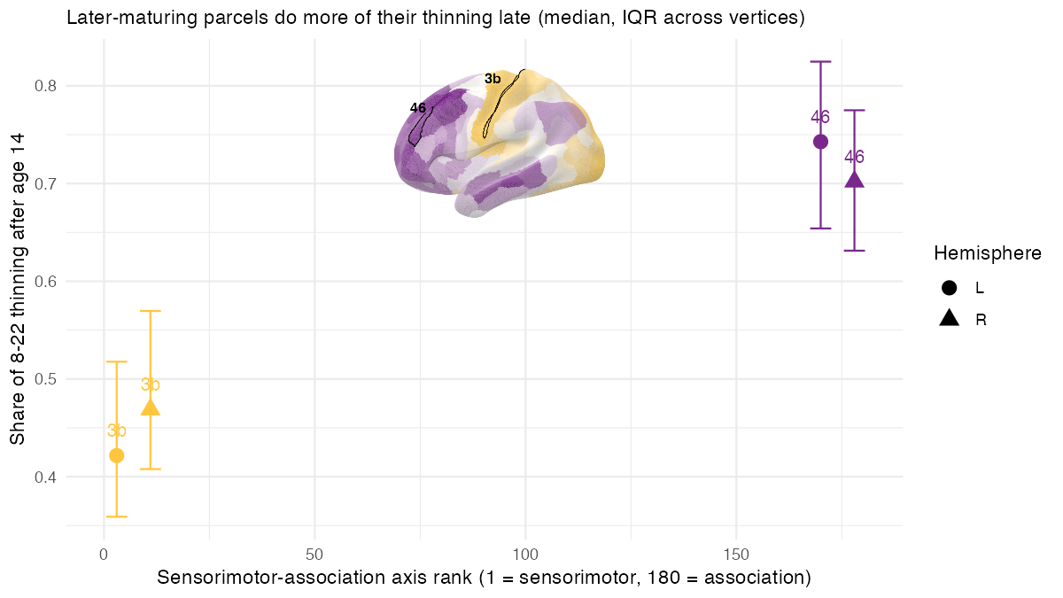
The literature check passes. Area 3b (sensorimotor) does most of its thinning early and area 46 (association) does most of its late: the share of the 8–22 thinning that happens after age 14 is about 0.4 in 3b and about 0.7 in 46 (Spearman ρ = 0.89 across the four parcel-hemispheres; age of fastest thinning ρ = 1.00):

Parcel	S-A rank	Late fraction (L / R)	Age of fastest thinning	Slope no longer clearly negative after
3b	7	0.41 / 0.48	5 y	19–23 y
46	174	0.74 / 0.71	23 y	still thinning at 23

Area 3b thins fastest in early childhood and is nearly flat by the late teens; area 46 thins slowly in childhood and fastest in the late teens and twenties — exactly the sensorimotor-first, association-last ordering of the S-A axis.

The S-A axis and the two parcels, in the colour scheme of Sydnor et al. (2021, Figure 2A) — gold at the sensorimotor pole, purple at the association pole:

How it works

Reaching the bucket. ModelArray uses the tiledb package’s default context. Set the region and anonymous access on it once, before ModelArray():

cfg <- tiledb::tiledb_config()
cfg["vfs.s3.region"] <- "us-east-1"
cfg["vfs.s3.no_sign_request"] <- "true"
tiledb::tiledb_ctx(cfg)

uri <- "s3://fcp-indi/data/Projects/RBC/RBC_FreeSurfer-Post_ModelArray/rbc_freesurferpost.tdb"
ModelArraySummary(uri)
ma <- ModelArray(uri, scalar_types = c("thickness", "curv"))

The environment variables TILEDB_VFS_S3_REGION and TILEDB_VFS_S3_NO_SIGN_REQUEST do the same thing. For a private bucket, use your usual AWS credentials instead of no_sign_request.

Tiles are the unit of cost. The store is dense float32, tiled as 964 vertices by all 8,696 sessions (33.5 MB before compression, 4–8 MB on the wire). Reading one vertex reads its tile, so element.subset ranges that fall in the same tile are nearly free, and a parcel whose vertices are spread over 20 tiles costs 20 tiles. The report prints this arithmetic before it reads, and caps each parcel at its most populated tiles.

One read pass per query. The tiledb R package reads a query in passes whose size is set by tiledb::set_allocation_size_preference() (10 MiB by default). Each pass re-fetches the tiles it touches, so with the default a 3-tile read can download 18 tiles. The report sets 512 MB; the report’s runtime table checks that the number of tiles read matches the prediction. This is separate from options(ModelArray.tiledb_read_block_mb), which controls how many elements ModelArray asks for at once (see vignette("large-scale-analyses")).

Results stay local. writeResults() writes to a local .h5 (or .tdb); the S3 store is never written to.

Why CovBat on a parcel at a time. Nine sites differ in both the mean and the spread of thickness, so a site covariate is not enough. CovBat harmonizes mean, variance and the covariance between features across sites. Harmonizing vertex by vertex inside the per-element function would work, but it is slow (one GAM fit per vertex just for the correction) and leaves nothing for the empirical-Bayes step to pool across. Reading a parcel’s vertices as one block and harmonizing them together is the method’s intended use, costs one covfam() call per parcel, and the harmonized block goes into a local HDF5 store that ModelArray reads like any other. Parcels are harmonized independently, so the report runs them in parallel, one per core (parallel::mclapply(); serially on Windows and on Binder). CovBat keeps every per-vertex GAM fit, so the report drops the copies of the data each fit carries, which covfam() never uses again; the harmonized values are unchanged, and each worker needs about 1 GB per 300 vertices. Repeat sessions (BHRC, NKI) are treated as independent, which the report says plainly and contrasts with a one-vertex longitudinal ComBat + GAMM fit.

One scalar at a time. ModelArray can attach a second scalar as an element-wise covariate when it lists the same source files as the phenotypes. In this store every scalar has its own file per session, so curv cannot ride along with thickness; the report uses thickness alone.

GAM choices. s(Age, k = 4) with REML, following PennLINC practice: a developmental curve needs at most two or three bends. Penalized p-values can be optimistic, so the test statistic comes from an fx = TRUE refit. Effect size is the change in adjusted R² when the smooth is dropped (what changed.rsq.term.index gives in ModelArray.gam()). Direction and timing come from the derivative of the fitted curve with a simultaneous interval (the same construction as gratia::derivatives()).

References

Bethlehem RAI et al. (2022). Brain charts for the human lifespan. Nature 604, 525–533.
Glasser MF et al. (2016). A multi-modal parcellation of human cerebral cortex. Nature 536, 171–178.
Sydnor VJ et al. (2021). Neurodevelopment of the association cortices. Neuron 109, 2820–2846.
Shaw P et al. (2008). Neurodevelopmental trajectories of the human cerebral cortex. J Neurosci 28, 3586–3594.
Tamnes CK et al. (2017). Development of the cerebral cortex across adolescence. J Neurosci 37, 3402–3412.
Chen AA et al. (2022). Mitigating site effects in covariance for machine learning in neuroimaging data. Hum Brain Mapp 43, 1179–1195. (CovBat)